1.2.3: Implementation

Once you have a formal model on paper, how do you turn it into code a computer can actually run, and what should you write down about that step so others can trust and reuse it? This section answers both questions, because a model that cannot be run, or cannot be reproduced from its description, is of little use to anyone.

Implementation is the stage at which the formal model is translated into code that a computer can execute. The modeller chooses a programming language or a dedicated modelling environment, represents each entity as an object with attributes and methods, represents the environment as a suitable data structure, and writes the simulation loop that advances the model one step at a time [1]. A good report of this stage explains the implementation without reproducing all of it. The parts worth reporting are:

What to report about the implementation

A good report explains the implementation without reproducing all of it. Click each part to see what is worth reporting.

This reporting guidance follows Nikolic, van Dam and Lukszo [1], with the Mesa framework used for the implementations throughout this book [2].

Two of those reporting choices, the tool used and the settings recorded, deserve a closer look before we make the guidance concrete, because they decide how easily the model can be built in the first place and whether its results can be trusted afterwards.

1.2.3.1: Choosing a modelling environment

The choice of modelling environment is not trivial. Nikolic, van Dam and Lukszo note that it shapes how easy it is to write the model, inspect it while it runs, and let other people reuse the code afterwards [1]. More specifically, the environment determines which kinds of agents, spaces, networks, activation schedules, and data collectors are readily available. It also affects how easily the modeller can trace an unexpected result back through the code, automate repeated experiments, connect the model to external data, and scale it to a larger population. A good fit between the formal model and the software therefore reduces translation work and makes assumptions easier to inspect; a poor fit can tempt the modeller to reshape the model around what the tool happens to support.

The decision still depends on practical constraints: what the modeller and team already know, the size and speed of the planned experiments, the analyses and visualisations required afterwards, and whether the project needs to integrate with other software. Familiarity can accelerate development, but it should be weighed against transparency, extensibility, documentation, community support, and the likelihood that the environment will remain usable. Section 1.4 compares these trade-offs and provides a structured route from modelling problem to paradigm and tool. Whichever environment is chosen, however, the same code can still be run in ways that others can or cannot repeat, and that is a matter of reproducibility.

1.2.3.2: Reproducibility of the implementation

Implementation choices also affect reproducibility, which is what lets a result be trusted and checked. Reproducing a result means reconstructing the conditions under which it was produced, not merely obtaining the same source-code file. The random seed, initial conditions, parameter values, activation order, stopping rule, and the moment at which output is collected can all change the outcome of a stochastic simulation. The software environment matters as well: the versions of Python, Mesa, and other dependencies may change defaults, algorithms, or numerical behaviour even when the model code itself is unchanged [1].

A reproducible implementation therefore stores these choices with the experiment, ideally in a configuration file or run record rather than only in prose. It should identify the code version, preserve the raw output needed to check reported figures, and explain any data-processing steps between the simulation and the final result. Fixed seeds are valuable for debugging and exact reruns, while multiple documented seeds are needed when the claim concerns the range or distribution of possible outcomes. This record benefits the original modeller as much as future readers: months later, it is the difference between being able to investigate a surprising result and having to guess how it was produced.

1.2.3.3: The traffic example: turning the formal model into code

With the tool and reproducibility settings in mind, we can now make this guidance concrete by working through how the running traffic model becomes code.

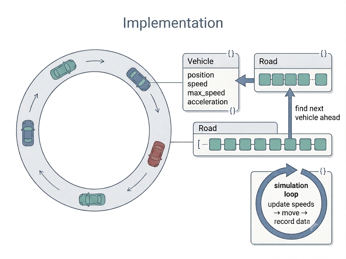
Fig. 7 Figure 1.7 Implementing the traffic model: each vehicle becomes a software object with its attributes, the road becomes a data structure linking each vehicle to the next, and a simulation loop updates every vehicle each step and records the output.

Implementing the traffic model means writing code that does the following. A vehicle becomes an object with attributes for position, speed, maximum speed, and any parameters such as acceleration and deceleration that vary between vehicles. The road becomes a data structure that stores the positions of all vehicles and lets each one find the next vehicle ahead. The simulation loop, at each step, asks every vehicle to update its speed according to the formal rules, then updates every vehicle’s position, and finally records the output the modeller needs, such as the speed of each vehicle at each step and the number of vehicles below some threshold speed.

A few implementation decisions follow directly from the formal model. The loop has to handle the fact that the road is a loop, so the vehicle at the front looks ahead to the vehicle at the back. The update order chosen at the formal stage has to be implemented exactly as specified, because updating all vehicles from a snapshot of the previous step can give different behaviour from updating them one at a time. When the model runs, the result is a sequence of states, where every vehicle is at every step and how fast it is moving, and that sequence is what verification, validation, and the simulation experiments will draw on [1].

1.2.3.3.1: Run the rule yourself

To see this translation in action, run the rule for yourself. The rule itself is short: each car looks at the gap to the car ahead, speeds up on open road but never past the speed limit, slows down when it is bunching up, and then moves forward by its current speed. The widget below sets that rule out as four numbered lines and runs it on a small ring of cars, where a slow patch soon appears even though nothing in the rule mentions one.

Learning Activity: Watch the rule run

see how a formal rule behaves once it is implemented and run.

Six cars sharing a one-lane ring road that wraps from the right edge back to the left, each car's colour showing its speed (red is slow, amber is medium, green is at the limit).

Press Step to run one tick at a time, or Play to run continuously (it becomes Pause), and watch the four numbered rule lines light up in order; press Reset to start over.

Tick: 0

Colour shows speed: stopped or slow medium at the limit

The car-following rule

1look at the gap to the car ahead

2if the gap is large, speed up, but never above the speed limit

3if the gap is small, slow down

4move forward by your current speed

Step Play Reset

NoteThis is implementation: the formal rule turned into lines a computer runs in order, one car and one step at a time. The stop-and-go bunching you see was never written into any single line. It comes out of every car running the same simple rule. Later in the chapter you will meet the fuller jam simulation, where the same idea drives a whole road.

Running the rule should have made one thing vivid: the stop-and-go patch of slow cars appears on its own, even though no single line of the rule ever tells a car to jam. That emergent bunching is exactly the kind of behaviour agent-based models are built to reveal, and the fuller jam simulation later in the chapter puts the same idea to work on a whole road.

1.2.3.3.2: From model parts to code forms

Watching one rule run also shows how orderly the translation is in general: each kind of element in the model has a natural counterpart in code. Entities become objects that carry their own attributes, the environment becomes a data structure, a behavioural rule becomes a method, one step of simulated time becomes one pass of the loop, and the quantities you want to study become recorded output. Seeing these correspondences clearly is what lets you move between a model on paper and a model in code without losing track of what each piece is doing. In the activity below, match each part of the traffic model to the code form it takes when the model is implemented.

Learning Activity: Match to code

connect each modelling idea to the code that expresses it.

Five parts of the traffic model, one per row, each turning into a particular code form when the model is implemented.

For every row, click the pill that names its code form, choosing from an object, a data structure, a loop pass, a method, and output data; once all five rows have a choice, press Check answers.

Check answers

Each part of the formal model had a natural home in the code. Once you can see those correspondences, implementation becomes a disciplined translation rather than a fresh act of invention.

With the model now running and producing a sequence of states, the next stage of the modelling cycle asks whether that code faithfully captures the formal model and whether the model itself is a trustworthy account of reality. Continue with Section 1.2.4 on verification and validation, which draws directly on the output the implementation produces.

Key takeaways

Key takeaways

• Implementation turns the formal model into running code: entities become objects, the environment becomes a data structure, and a simulation loop advances the model step by step.

• The report should explain the tool, code structure, key algorithms, and data structures, not reproduce the whole program.

• Recording the random seed, software version, and parameter values is what makes a result reproducible.

References

[1] (1,2,3,4,5)

Nikolic, I., van Dam, K. H., & Lukszo, Z. (2013). Practice. In K. H. van Dam, I. Nikolic, & Z. Lukszo (Eds.), Agent-based modelling of socio-technical systems (pp. 73–137). Springer.

[2]

Kazil, J., Masad, D., & Crooks, A. (2020). Utilizing Python for agent-based modeling: The Mesa framework. In R. Thomson, H. Bisgin, C. Dancy, A. Hyder, & M. Hussain (Eds.), Social, cultural, and behavioral modeling (SBP-BRiMS 2020), LNCS 12268 (pp. 308–317). Springer.