

2.2.2: Environment and space#
In a nutshell
What is the environment in an agent-based model, and what choices define it? This section works through four connected questions: what role the environment plays, what kinds of environment exist, how it changes over time, and what spatial medium (the space) sits inside it. Getting these choices right matters because the environment is not scenery: it decides what agents can sense, where they can go, and who they can reach.
2.2.2.1: Role of the environment#
The environment is the world the agents live in, the context that surrounds them and gives their actions meaning. Agents cannot exist in a vacuum: they must be placed somewhere, they sense and change what is around them, and the environment supplies both the information they act on and the structure that decides who can reach whom. This matters when you build a model because the environment is not mere scenery; it actively shapes what the agents can do and therefore what the whole system can produce. In the panel below, each card gives one reason the environment matters. Click each to expand it, and notice that the reasons are not separate points but different faces of the same idea, that behaviour only makes sense in a setting.
The lesson to carry away is that the environment is an active part of any model, not a backdrop, because it supplies the information agents use and the structure that governs their interactions. Once you accept that it is active, the first modelling choice is what kind of environment it is.
2.2.2.2: Examples of different types of environments#
An environment is a bundle of assumptions about geometry and access. A square or hexagonal grid makes location discrete and defines movement through neighbouring cells; continuous space allows arbitrary coordinates and metric distance; a network replaces physical proximity with links; and Voronoi space divides an irregular landscape into regions. These choices determine who can meet, what an agent can sense, whether several agents may share a place, and how quickly influence can travel. The most visually realistic environment is not automatically the best one. The right choice is the simplest structure that preserves the relationships needed for the research question[1].
The activity below lets you compare how these environments organise location and neighbourhoods.
2.2.2.3: Neighbourhoods on a grid#
Of the three spaces just introduced, the grid deserves a closer look because it forces one further choice that the others do not: which nearby cells count as “near”. On a grid, much of an agent’s behaviour depends on its neighbourhood, that is, the set of cells it can sense or affect. There is more than one way to define that neighbourhood: the four cells sharing an edge (the von Neumann neighbourhood), the eight cells that also share a corner (the Moore neighbourhood), or a wider ring reaching further out. This choice matters because it fixes how far local influence travels in a single step, and so how quickly things spread across the grid. In the tool below, pick a definition and click any cell to light up its neighbours, and watch how the count falls near the edges, where cells have fewer neighbours than those in the middle.
The lesson to keep is that the neighbourhood you choose quietly sets the reach of every local interaction, and the edges of a grid behave differently because cells there simply have fewer neighbours.
The explorer above showed which cells count as neighbours; the activity below sets that neighbourhood in motion, letting the same spreading process run on three different grids so the consequences of the choice become visible.
OrthogonalVonNeumannGrid, OrthogonalMooreGrid, or HexGrid, together with the neighbourhood radius, and the choice changes what the model does.The lesson is that the neighbourhood definition and the grid topology are deliberate modelling choices, not incidental details: in Mesa they correspond to OrthogonalVonNeumannGrid, OrthogonalMooreGrid, and HexGrid together with the neighbourhood radius, and each reshapes how quickly and in what pattern influence travels across the space.
2.2.2.4: Worked example: space shapes dynamics (virus on a network)#
Neighbourhoods showed how a spatial choice sets the reach of interaction on a grid; the same principle holds for a network space, where the pattern of connections sets who can reach whom. The type of network space can dramatically affect how phenomena such as disease spread through a population. In the virus on a network model, different network topologies create different patterns of transmission:
Network topology types:
Newman-Strogatz: Small-world networks with high clustering but short path lengths
Barabasi-Albert: Scale-free networks with a few highly connected hubs
Complete: Every agent is connected to every other agent
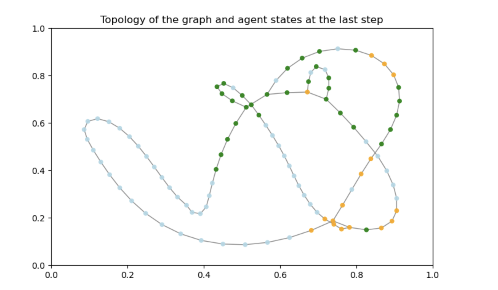
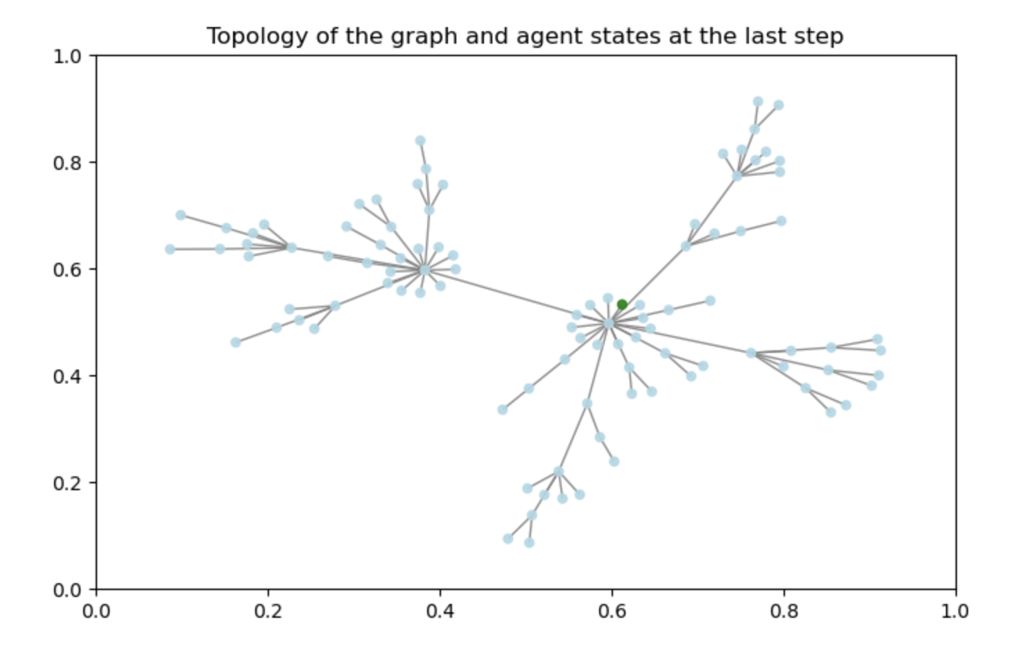
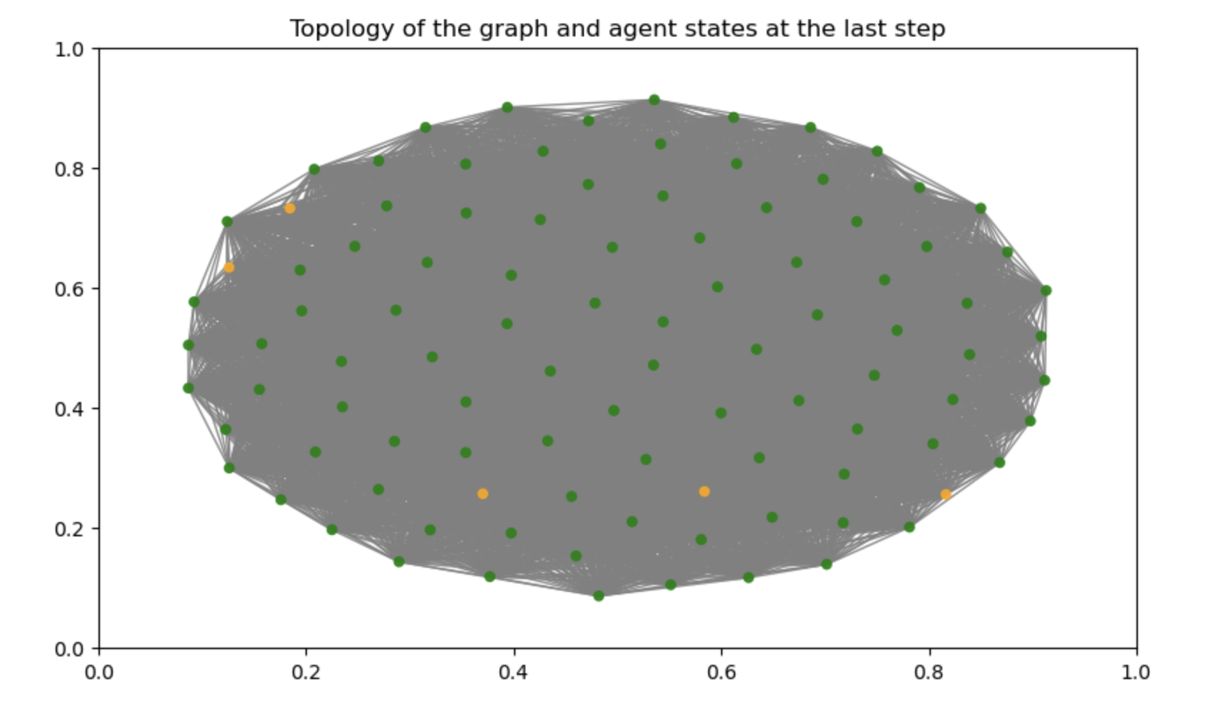
Each topology affects how quickly and how widely the virus spreads through the population. This demonstrates how the choice of spatial structure, that is, the network type, fundamentally shapes system dynamics in ABM.
The static figures above show the finished patterns; the activity below lets you predict them before they form. The same virus, the same rule, three different network shapes. Before you begin, predict which one it races through fastest.
The lesson to carry away is that the same virus and the same rule can spread quickly or slowly depending only on the shape of the network, which is why the environment, and not just the agents, decides what happens.
Pulling the four axes together, the environment is the situated, active part of a model, and the space is the structural medium within it that decides who can reach whom. With the environment and its space in place, the next section turns to how agents act within it over time.
Key takeaways#
Key takeaways
The environment situates the agents and supplies the context and information they perceive and act upon.
The type of space, whether a grid, a network, or geographic coordinates, determines which agents can interact, and therefore shapes the patterns that emerge.
The environment is not static: it can change over time and in response to agent behaviour, feeding back into subsequent decisions.