import matplotlib
if not hasattr(matplotlib.RcParams, "_get"):
    matplotlib.RcParams._get = dict.get

4.1.1: Exercises

Important

For live code, launch Thebe by clicking on the in the toolbar. Your code edits are automatically saved in your browser. Use the button to export your progress to a file, to import a previously saved session, or to reset to the original code.

4.1.1.1: The base model

Attention

This model is up-to-date with mesa version 3.5.0

%pip install mesa==3.5.0
%pip install seaborn
%pip install networkx

4.1.1.1.1: Understanding the simple economy model

import mesa

# Print the version of the mesa library being used
print("You are using mesa version: " + mesa.__version__)

# Import the base Agent and Model classes from mesa
from mesa import Agent, Model

# Import the DataCollector for collecting data during the simulation
from mesa.datacollection import DataCollector

# Import matplotlib for plotting
import matplotlib.pyplot as plt

# Import numpy for numerical operations and useful math functions
import numpy as np

# Import seaborn for enhanced data visualization
import seaborn as sns

# For Jupyter Notebook: ensure matplotlib draws graphs inline
%matplotlib inline

# Import the statistics module for basic statistical operations
import statistics as stat

# Import pandas for data manipulation and analysis
import pandas as pd

# Import required libraries for animation
from matplotlib.animation import FuncAnimation  # Animation functions from matplotlib
from IPython.display import HTML  # Display tools for rendering animations in Jupyter Notebooks

You are using mesa version: 3.5.0

Agent class

"""
The `MoneyAgent` class represents an individual agent in the economy. 
Each agent has an initial wealth and a maximum amount of money they can 
take from another agent. In each step, an agent randomly selects another 
agent and takes a random amount of money from them, up to the maximum limit. 
If the other agent has enough money, it is deducted from their wealth and added 
to the wealth of the current agent. If the other agent does not have enough money,
the current agent takes all the money the other agent has.
"""
class MoneyAgent(Agent):
    """ An agent with fixed initial wealth."""
    
    def __init__(self, model, max_init_money, max_take_money):
        """Initialize a MoneyAgent with given attributes."""
        super().__init__(model)  # Initialize the parent Agent class
        self.wealth = self.random.randrange(max_init_money)  # Set initial wealth to a random value
        self.max_take_money = max_take_money  # Set the maximum money the agent can take

    def step(self):
        """Define the agent's behavior for one step."""
        
        other_agent = self.random.choice(self.model.agents)  # Randomly select another agent
        money_to_take = self.random.randrange(self.max_take_money)  # Determine a random amount of money to take
        
        # Determine how much the other agent has
        available_to_take = other_agent.wealth
        
        # Check if the other agent has enough money
        if available_to_take >= money_to_take:
            other_agent.wealth -= money_to_take  # Deduct the money from the other agent
            self.wealth += money_to_take  # Add the money to this agent's wealth
        else:  # If the other agent does not have enough money
            self.wealth += available_to_take  # Take all the money the other agent has
            other_agent.wealth -= available_to_take  # Set the other agent's wealth to zero

Model class

"""
The `MoneyModel` class represents the overall model of the economy. 
It initializes a specified number of agents and sets their maximum initial wealth
 and maximum amount of money they can take. The model progresses in steps, where 
 each step activates all the agents in the model randomly, allowing them to interact 
 with each other and exchange money.

These classes provide the foundation for simulating wealth distribution and dynamics
in the economy.
"""
class MoneyModel(Model):
    """A model with some number of agents."""
    
    def __init__(self, N, max_init_money=100, max_take_money=10):
        """Initialize the MoneyModel with a specified number of agents."""
        super().__init__()  # Explicitly call the superclass's __init__ method
        self.num_agents = N  # Set the number of agents in the model
        
        # Create agents
        MoneyAgent.create_agents(
            model=self, 
            n=self.num_agents,
            max_init_money=max_init_money,
            max_take_money=max_take_money
        )

    def step(self):
        """Advance the model by one step."""
        self.agents.shuffle_do("step") # Activate step for each agent in random order

Before moving on, it is worth pinning down which of these two classes owns each piece of the model.

Learning Activity: Agent class or model class?

separate what one participant owns from what the whole economy owns.

Three flip cards contrasting what the MoneyAgent class owns for a single participant, what the MoneyModel class owns for the whole economy, and where the boundary between them lies.

Click each card to flip it and reveal exactly what lives inside that class in the base model.

A MoneyAgent knows only itself: its own wealth, its max_take_money, and how to take money in step(). A MoneyModel knows everyone: it stores num_agents, builds the population, and decides who acts and when. Keeping that boundary clear is what makes an agent-based model easy to reason about.

Holding that boundary in mind, individual state and behaviour in the agent and population-level control in the model, is the single most useful habit when reading or writing any Mesa model.

Task: convert the base model into a flow chart

Convert the base model into a flow chart that tells a story of what is going on. You may use pen and paper for this.

Before drawing your own flow chart, try assembling the model’s execution order from its shuffled steps below.

Learning Activity: Order the model loop

reconstruct one run of the simple economy from setup to stop.

The six steps of a full MoneyModel run, from initial setup through the repeating tick loop, presented in a shuffled pool.

Click each step in turn to drop it into the numbered slots in the order it executes, click a placed chip to send it back, and once all six slots are full press Check order.

Your order

Steps (click to place)

Check orderReset

Notice that only the setup happens once while the middle steps repeat every tick, which is exactly the loop your flow chart needs to capture.

Solution

To create a flowchart that represents the base agent-based model, you can follow these steps:

1. Start:

   • Begin the flowchart with an oval labeled “Start.”

2. Initialise the Model:

   • Process Box: Draw a rectangle labeled “Initialise MoneyModel with N agents.”

   • Process Box: Add another rectangle labeled “Set max initial wealth and max money to take.”

   • Process Box: Draw a rectangle labeled “Create MoneyAgents for the model.”

3. Main Loop:

   • Decision Box: Draw a diamond labeled “Has the Termination Condition Been Met?” (e.g., fixed number of steps).

     • Yes Path: Draw an arrow from this decision box to an oval labeled “End”.

     • No Path: If the termination condition isn’t met, continue to the next steps in the loop.

4. Step 1: Agent Interaction:

   • Process Box: Draw a rectangle labeled “Randomly select another agent”.

   • Process Box: Draw a rectangle labeled “Determine random amount of money to take (up to max limit)”.

5. Step 2: Wealth Exchange:

   • Decision Box: Draw a diamond labeled “Does the other agent have enough money?”.

     • Yes Path:

       • Process Box: Draw a rectangle labeled “Deduct the money from the other agent”.

       • Process Box: Draw a rectangle labeled “Add money to the current agent’s wealth”.

     • No Path:

       • Process Box: Draw a rectangle labeled “Take all available money from the other agent”.

       • Process Box: Draw a rectangle labeled “Set the other agent’s wealth to zero”.

6. Step 3: Update Agents:

   • Process Box: Draw a rectangle labeled “Activate all agents in the model for one step randomly”.

7. Repeat Loop:

   • Draw an arrow from “Activate all agents in the model for one step randomly” back to the main loop’s decision box labeled “Has the Termination Condition Been Met?”.

   • This indicates the repetition of the loop until the termination condition is satisfied.

8. End:

   • When the termination condition is met, direct the flow to an oval labeled “End”.

Summary:

1. Start -> Initialise MoneyModel -> Create Agents -> (Loop Start) Has the Termination Condition Been Met? -> No -> Randomly Select Another Agent -> Determine Random Amount -> Does the Other Agent Have Enough Money? -> Yes -> Deduct Money -> Add to Current Agent’s Wealth -> Activate Agents -> (Loop Back to Condition Check) -> Yes -> End

Draw the flowchart: You can use pen and paper or software tools like Google Drawings or Lucidchart.

4.1.1.1.2: Running the model

# Create an instance of the MoneyModel class with 1000 agents. 
# In object-oriented programming, a class is a blueprint or template for creating objects,
# and an instance refers to a specific occurrence or realization of that class.
# In this case, the `MoneyModel` class represents the overall model of the economy,
# and the `model` variable stores an instance of this class.
# The seed parameter is optional but enables reproducible results.

model = MoneyModel(1000)

# Run the model for a specified number of steps.
# In this case, the model is run for 100 steps.
# This loop activates all the agents in the model for 100 steps.
# The `step()` method of the model advances the model by one step,
# which, in turn, activates all the agents randomly for one step.
# The `step()` method is defined in the `MoneyModel` class.

for i in range(100):
    model.step()

Task: change number of agents and runs

Change the following and Run the model above:

• Run the model above with a different number of agents. try 10,100, 1000

• Does increasing the number of agents affect the simulation time?

• Run the model above with a different number of runs. Try 10,100, 1000

• Does increasing the number of runs affect the simulation time?

• Reset the original values (number of agents = 1000 and number of runs = 100) and then proceed to the following section

# answer here

Solution

For this task, you will experiment with how changing the number of agents and the number of runs affects the simulation time. Follow the steps below:

• Change the number of agents: Modify the number of agents when creating the MoneyModel. Try setting the number of agents to 10, 100, 1000, and 10000.

  • You can do this by replacing the value in the MoneyModel(1000) call with each number you want to test, for example, MoneyModel(10) for 10 agents.

  Hint: If you are unsure how to measure time, Python’s time module can be used to check how long the model takes to run. Place start_time = time.time() before the simulation loop, and end_time = time.time() after it. The difference will give you the total runtime.

• Run the simulation: Use a loop to run the model for each of the agent counts. Record the time it takes for each simulation.

  • You can structure this with a simple for loop, running the model for each agent count and measuring the time.

• Does increasing the number of agents affect the simulation time?: After running the simulations for each agent count, compare the time it takes. Hint: You should notice that as the number of agents increases, the simulation might take longer. This happens because the model has more agents to process.

• Change the number of runs: After testing different agent counts, change the number of simulation runs. You can do this by modifying the range in the loop, e.g., from range(100) to range(10) and range(1000)

  Hint: Make sure you are only changing the number of runs (iterations) this time and keeping the number of agents fixed, so you can isolate the effect of changing the number of runs on simulation time.

• Does increasing the number of runs affect the simulation time?: Like before, compare the time it takes for each set of runs. Increasing the number of runs should also increase the simulation time.

• Reset values: Once you’ve gathered your data, return the number of agents to 1000 and the number of runs to 100, as it was in the original setup.

4.1.1.1.3: Storing the results

# Lets collect some data about the model, now that we finished running it.

# Create a list to store the wealth of each agent
agent_wealth = [a.wealth for a in model.agents]

# The above line uses a list comprehension to iterate over each agent in the model
# and retrieve their wealth using the `wealth` attribute of the `MoneyAgent` class.
# The retrieved wealth values are then stored in the `agent_wealth` list.

# Print the wealth of each agent after running the model
print(agent_wealth)

[31, 80, 61, 8, 132, 27, 138, 75, 29, 78, 47, 107, 10, 87, 17, 78, 27, 108, 83, 26, 65, 68, 54, 16, 41, 7, 71, 0, 28, 3, 35, 55, 117, 67, 5, 82, 12, 6, 6, 0, 118, 40, 148, 16, 81, 150, 68, 41, 82, 1, 57, 71, 23, 10, 34, 81, 72, 29, 33, 95, 58, 0, 11, 8, 94, 4, 93, 80, 0, 6, 11, 11, 31, 108, 46, 1, 5, 37, 15, 46, 68, 85, 6, 29, 5, 166, 83, 12, 122, 63, 115, 107, 75, 0, 0, 22, 21, 87, 80, 25, 124, 18, 153, 4, 32, 18, 43, 18, 4, 93, 22, 8, 130, 4, 43, 38, 76, 123, 2, 40, 140, 30, 36, 48, 27, 27, 47, 3, 22, 27, 60, 8, 15, 28, 65, 115, 94, 19, 95, 2, 54, 13, 97, 36, 30, 57, 100, 17, 4, 97, 138, 32, 26, 85, 40, 82, 9, 105, 18, 0, 36, 23, 32, 64, 77, 34, 39, 26, 58, 22, 20, 53, 32, 131, 167, 106, 99, 70, 66, 24, 22, 39, 0, 81, 52, 5, 22, 135, 61, 4, 14, 3, 46, 43, 25, 51, 92, 15, 23, 13, 130, 57, 8, 26, 63, 51, 7, 17, 57, 13, 95, 53, 76, 65, 42, 74, 125, 44, 41, 164, 39, 75, 72, 85, 20, 9, 6, 7, 72, 16, 37, 8, 64, 61, 44, 15, 1, 17, 12, 16, 8, 41, 80, 146, 53, 108, 105, 28, 28, 7, 13, 7, 56, 72, 51, 46, 1, 78, 29, 7, 13, 45, 15, 94, 21, 132, 79, 0, 58, 14, 30, 18, 117, 33, 0, 34, 22, 52, 122, 40, 123, 99, 77, 105, 30, 87, 48, 115, 40, 21, 86, 6, 6, 64, 24, 64, 110, 20, 132, 20, 50, 24, 62, 90, 47, 81, 8, 18, 89, 241, 68, 109, 191, 112, 46, 69, 97, 48, 165, 17, 19, 126, 94, 226, 13, 31, 17, 11, 34, 63, 8, 24, 63, 65, 166, 10, 0, 137, 13, 101, 3, 7, 2, 70, 90, 39, 20, 39, 3, 0, 19, 29, 72, 22, 44, 116, 19, 86, 37, 45, 15, 24, 74, 71, 10, 11, 64, 70, 44, 115, 10, 0, 67, 26, 103, 5, 32, 52, 95, 86, 68, 25, 42, 129, 124, 44, 4, 0, 28, 44, 22, 115, 25, 1, 35, 63, 41, 24, 8, 120, 40, 25, 53, 13, 11, 67, 42, 170, 52, 22, 2, 13, 6, 85, 30, 11, 113, 48, 38, 1, 57, 10, 28, 96, 8, 66, 13, 28, 137, 120, 43, 59, 1, 3, 77, 44, 62, 25, 36, 49, 45, 44, 9, 105, 97, 24, 48, 18, 82, 33, 115, 53, 0, 44, 106, 112, 97, 58, 16, 199, 61, 54, 55, 36, 11, 91, 46, 70, 21, 57, 1, 50, 7, 33, 4, 9, 55, 59, 12, 50, 24, 37, 35, 34, 115, 88, 47, 4, 31, 31, 7, 83, 0, 80, 25, 32, 23, 107, 18, 0, 4, 99, 163, 12, 139, 40, 16, 62, 51, 9, 27, 0, 68, 19, 186, 52, 17, 147, 7, 42, 85, 35, 114, 11, 21, 8, 18, 20, 54, 32, 11, 79, 70, 35, 24, 21, 6, 74, 74, 108, 100, 18, 97, 9, 0, 76, 59, 13, 68, 180, 0, 37, 92, 18, 123, 217, 34, 45, 11, 67, 15, 25, 5, 114, 14, 63, 14, 37, 2, 112, 82, 13, 12, 32, 102, 101, 0, 6, 5, 30, 10, 29, 62, 130, 43, 0, 61, 19, 9, 2, 33, 30, 77, 37, 34, 190, 98, 117, 65, 111, 1, 78, 27, 10, 80, 0, 12, 25, 11, 96, 0, 38, 27, 12, 3, 14, 51, 41, 21, 56, 71, 9, 20, 0, 45, 83, 44, 17, 139, 40, 5, 3, 56, 18, 49, 0, 24, 22, 15, 63, 136, 8, 9, 23, 56, 4, 4, 19, 31, 46, 84, 43, 66, 37, 3, 23, 5, 117, 50, 11, 106, 100, 5, 36, 96, 9, 58, 6, 99, 21, 88, 89, 7, 5, 58, 59, 6, 63, 60, 154, 26, 12, 37, 41, 22, 88, 177, 53, 0, 18, 89, 31, 45, 27, 125, 72, 23, 102, 10, 72, 49, 47, 7, 15, 54, 20, 82, 136, 29, 25, 30, 103, 29, 34, 41, 72, 68, 0, 10, 95, 5, 17, 123, 91, 25, 30, 64, 24, 72, 9, 6, 6, 28, 68, 17, 15, 74, 101, 128, 96, 125, 55, 25, 36, 59, 17, 62, 27, 3, 17, 48, 25, 32, 98, 21, 35, 92, 62, 83, 12, 1, 177, 28, 98, 23, 0, 76, 54, 100, 1, 113, 71, 37, 18, 46, 25, 39, 34, 40, 31, 61, 34, 95, 23, 5, 4, 6, 98, 40, 12, 91, 0, 88, 15, 4, 50, 65, 3, 138, 17, 44, 44, 141, 16, 11, 33, 6, 17, 8, 10, 70, 51, 40, 35, 48, 105, 27, 49, 8, 11, 13, 55, 0, 95, 15, 54, 3, 27, 2, 22, 96, 0, 73, 46, 132, 72, 109, 148, 17, 38, 80, 14, 88, 12, 18, 37, 9, 2, 24, 133, 35, 144, 57, 51, 17, 54, 69, 27, 29, 0, 19, 181, 43, 0, 31, 32, 40, 11, 71, 61, 17, 45, 30, 49, 89, 64, 10, 5, 22, 11, 5, 24, 77, 67, 45, 33, 22, 72, 20, 8, 42, 55, 56, 18, 23, 21, 8, 20, 67, 80, 35, 69, 98, 57, 42, 124, 71, 10, 111, 42, 57, 82, 10, 28, 104, 40, 95, 44, 48, 50, 20, 4, 97, 47, 54, 22, 25, 8, 42, 54, 126, 102, 48, 17, 57, 43, 29, 4, 89, 41, 9, 20, 14, 36, 129, 71, 50, 102, 115, 15, 48, 12, 96, 40, 123, 0, 94, 53, 165, 11, 92, 18, 86, 23, 85, 52, 19, 75, 13, 87, 95, 98, 137, 61, 14, 138, 94, 107, 50, 17, 136, 12, 15, 147, 40, 84, 76, 23, 74, 0, 8, 6, 77, 47, 27, 7, 92, 30, 16, 38]

Task: interpret the results of the agent_wealth

Please write up to 5 sentences in your own words:

• Describe results of the agent_wealth. What does each value in the list represent?

• Can you identify any sort of agents or model behaviour without visualising the results?

Solution

Now that we’ve collected the wealth data for each agent, let’s interpret what this list represents.

• The agent_wealth list contains the wealth of each agent after the simulation has run. Each value in the list corresponds to the amount of money an individual agent has at the end of the simulation. You can think of each value as representing an agent’s final “financial status” within the model’s economic system.

• The wealth distribution among agents is typically not uniform. Some agents may accumulate more wealth, while others might end up with little to none.

• Without visualising the data, you may notice patterns such as agents losing all their wealth while others accumulate it over time. This is likely due to the random nature of interactions between agents, where some agents consistently take wealth from others, leading to inequality in wealth distribution. Note that it is difficult to interpret a large dataset without visualisation. We will visualise the results later in this notebook.

4.1.1.2: Model output

4.1.1.2.1: System-level properties at the end of the simulation

Exercise: statistical measures

• Determine the following statistical measures of the agent population’s wealth:

  • Maximum wealth

  • Minimum wealth

  • Mean wealth

  • Median wealth

  • Mode of wealth

• What observations can you make from these measures?

Hint: You can use the statistics library.

# answer here

Solution

# Calculate the minimum, maximum, mean, median, and modal wealth of the population
print("Minimum money of the population = " + str(min(agent_wealth)))  # Calculate and print the minimum wealth of the population
print("Maximum money of the population = " + str(max(agent_wealth)))  # Calculate and print the maximum wealth of the population
print("Mean money of the population = " + str(stat.fmean(agent_wealth)))  # Calculate and print the mean wealth of the population using the fmean() function from the statistics module. f mean is used to avoid floating point errors. 
print("Median money of the population = " + str(stat.median(agent_wealth)))  # Calculate and print the median wealth of the population using the median() function from the statistics module
print("Modal money of the population = " + str(stat.mode(agent_wealth)))  # Calculate and print the mode of the wealth distribution in the population using the mode() function from the statistics module

Exercise: create a histogram

• Now, create a histogram of the money held by agents.

• What observations can you make from the histogram?

# answer here

Solution

# This code cell uses the seaborn library to create a histogram of the agent_wealth data.
# sns.histplot(agent_wealth): Plots the distribution of wealth among agents.
# For more on seaborn, visit the Seaborn Documentation: (https://seaborn.pydata.org/).

sns.histplot(agent_wealth)

4.1.1.2.2: Effect of simulation time on the end state

The final outcome of a simulation depends on its duration. Longer simulations allow more changes to accumulate, leading to different end states. This is because dynamic systems evolve over time, and their state at any point is influenced by the length of the simulation. Consequently, varying the duration can capture different phases of the system’s behaviour, from transient to steady state.

Exercise: check the state of the simulation using a histogram

• Check the state of the simulation at 0,2,5,10,100,500 steps, using a histogram.

• What do you notice ?

# answer here

Solution

#initialize a new model with 100 agents
model = MoneyModel(100)

# Timesteps to collect the data about the model. 
# We will collect data at the following timesteps: 0, 2, 5, 10, 100, 500
steps_to_measure = [0,2,5,10,100,500]

for i in range(501): # Run the model for 501 steps. 501 is used to include the last step in the list of steps to measure because 0 is counted as one step.
    if i in steps_to_measure: # Check if the current step is in the list of steps to measure
        agent_wealth = [a.wealth for a in model.agents]  # Collect the wealth of each agent in a list
        plt.figure() # Create a new figure for plotting
        sns.histplot(agent_wealth)  # Create a histogram of the agent wealth distribution
        plt.title("Wealth distribution at t = " + str(model.steps))  # Set the title of the histogram
        plt.xlabel("Agent wealth")  # Set the x-axis label
        plt.ylabel("Number of agents")  # Set the y-axis label
    model.step()  # Advance the model by one step


# We notice that the distribution become more unequal over time.
# The number of agents with low wealth increases, while the number of agents with high wealth decreases.

Before turning to the exercises, the lab below lets you drive the very same economy yourself. Every agent starts with an identical purse, and on each step every agent that still has money gives one unit to another agent chosen at random. Nothing here favours anyone, yet the shape of the outcome is anything but even.

Learning Activity: The inequality lab

watch how population size and run length shape the final wealth distribution and its Gini.

A wealth-exchange simulation in which every agent starts with the same fifteen coins and, each step, gives one coin to another agent picked at random.

Drag Steps to advance time or press Play to run the model, then change the Number of agents to test whether population size matters, keeping an eye on the Gini readout.

Gini

0.00

Mean

15

Richest

15

Broke

0%

agents at each wealth levelstarting wealth (15)

wealth per agent, from poorest (left) to richest (right)

Number of agents120

Steps0

PlayReset

At step 0 every agent is equal, so the histogram is a single tall spike and the Gini is 0.

This is the same wealth-exchange rule as the MoneyModel you have been running. Because money performs a random walk with no force pulling it back to the average, an equal start relaxes into a skewed, roughly exponential distribution, and the Gini climbs from 0 towards about 0.5 and settles there. The final shape barely depends on how many agents there are, but it depends strongly on how long the model runs: inequality here is an emergent property of time and chance, not of any unfair rule.

The point to carry into the exercises is that a fair, symmetric rule still produces lasting inequality, and that the amount of inequality is set mainly by how long the model runs, not by how many agents take part.

4.1.1.2.3: System-level properties over time

Next, we want to study the behaviour of the entire system over the course of the simulation run. One way to do this is by creating a movie of the wealth histogram throughout the entire simulation. This allows us to visualise how the distribution of wealth changes over time and gain insights into the dynamics of the system.

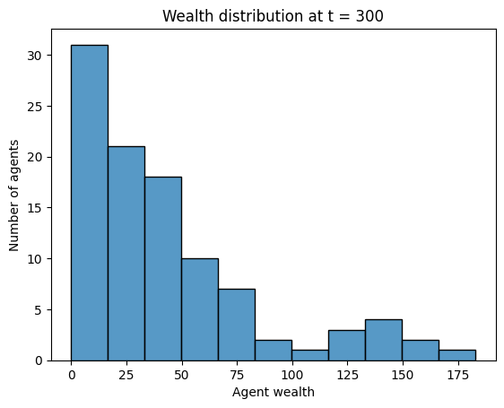
Let’s proceed with creating the movie of the wealth histogram over the entire simulation run of 300 steps.

# Here we will be using a matplotlib function called FuncAnimation: https://matplotlib.org/stable/api/_as_gen/matplotlib.animation.FuncAnimation.html
# It will repeatedly call the update function on the figure object we have given it.
# We are using it in a similar way we used our for loop in the previous step.

# Initialize a new model
model = MoneyModel(100)

# Get the initial wealth statistics of the agents
agent_wealth = [a.wealth for a in model.agents]

# Create a figure to draw on
fig = plt.figure()

# The update function. This function is called every time we take a step in the animation
def update(frame):
    # Clear the previous image, since the plt.hist() function does not have an update method like some others
    plt.cla() 
    
    # Compute the wealth statistics of the agents
    agent_wealth = [a.wealth for a in model.agents]
    
    # Make the plot
    sns.histplot(agent_wealth)
    
    # Make the plot visually appealing
    plt.title("Wealth distribution at t = " + str(model.steps))
    plt.xlabel("Agent wealth")
    plt.ylabel("Number of agents")
    
    # Step the model. We are stepping the model only after we have done the plot, so that we can capture step 0
    model.step()
    

# Create the animation using the update function, updating every 100 milliseconds for 300 frames
anim = FuncAnimation(fig, update, interval=100, frames=299) #frame 1 is automatically created by the initial plot so the total number of frames is 300

# Display the animation as an interactive JavaScript player.
# to_jshtml() renders the frames with JavaScript, so it works everywhere, including live code in the browser, with no ffmpeg needed.
plt.rcParams['animation.embed_limit'] = 2**128  # allow the player to embed all frames
HTML(anim.to_jshtml())
# If you are running the notebook locally and have ffmpeg installed, you can instead render a compact HTML5 video:
# HTML(anim.to_html5_video())

# Now add a second plot to the movie, plotting the wealth of the richest agent

# Initialize a new model with 100 agents
model = MoneyModel(100)

# Get the initial wealth statistics of the agents
agent_wealth = [a.wealth for a in model.agents]

# Create a list to store the wealth of the richest agent at each time step
richest_agent_wealth = [max(agent_wealth)]

# Create a list to store the time steps
steps = [model.steps]

# Create a figure with 2 subplots, and set the size to 4x4 inches and the resolution to 200 dpi
fig, (ax1, ax2) = plt.subplots(2, figsize=(4, 4), dpi=200)

# Add padding between the subplots for better visualization
fig.tight_layout(pad=5.0)

# Create an initial empty line plot for the wealth of the richest agent over time
sns.lineplot(x=steps, y=richest_agent_wealth, ax=ax2)

# The update function. This function is called every time we take a step in the animation
def update(frame):
    # Clear the previous plots by resetting the axes
    ax1.cla()
    ax2.cla()
    
    # Compute the wealth statistics of the agents at the current time step
    agent_wealth = [a.wealth for a in model.agents]
    
    # Add the current richest agent's wealth to the list
    richest_agent_wealth.append(max(agent_wealth))
    # Add the current time step to the list
    steps.append(model.steps)
    
    # Plot the wealth distribution of all agents as a histogram
    sns.histplot(agent_wealth, ax=ax1)
    # Set the title of the histogram plot to indicate the current time step
    ax1.set_title("Wealth distribution at t = " + str(model.steps))
    # Set the x-axis label of the histogram plot
    ax1.set_xlabel("Agent wealth")
    # Set the y-axis label of the histogram plot
    ax1.set_ylabel("Number of agents")
    
    # Plot the wealth of the richest agent over time as a line plot
    ax2.set_title("Wealth of the richest agent")
    ax2.set_xlabel("Timesteps")
    ax2.set_ylabel("Agent wealth")
    sns.lineplot(x=steps, y=richest_agent_wealth, ax=ax2)
    
    # Step the model to the next time step, updating the state of all agents
    model.step()

# Create the animation using the update function, updating every 100 milliseconds for 300 frames
anim = FuncAnimation(fig, update, interval=100, frames=299) #frame 1 is automatically created by the initial plot so the total number of frames is 300

# Display the animation as an interactive JavaScript player.
# to_jshtml() renders the frames with JavaScript, so it works everywhere, including live code in the browser, with no ffmpeg needed.
plt.rcParams['animation.embed_limit'] = 2**128  # allow the player to embed all frames
HTML(anim.to_jshtml())
# If you are running the notebook locally and have ffmpeg installed, you can instead render a compact HTML5 video:
# HTML(anim.to_html5_video())

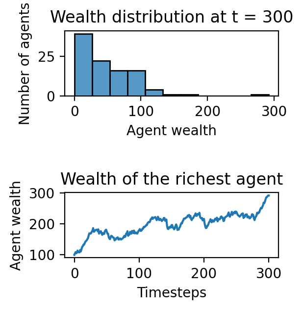
Task: describe the behaviour of the agents as shown in the provided animation/plot

Please write up to 5 sentences in your own words:

• Describe what you see in the provided animation/plot.

• Describe the behaviour of the agents as shown in the provided animation/plot.

• What patterns, trends, or interactions do you observe among the agents throughout the simulation?

Solution

Looking at the animation/plot, you can observe the following patterns:

• Over time, the wealth distribution among agents becomes increasingly unequal. In the early stages, wealth is more evenly distributed, but as the simulation progresses, fewer agents hold most of the wealth while the majority have less.

• The behaviour of the agents shows a clear tendency toward wealth concentration. As the steps increase, a few agents consistently accumulate more wealth, while many agents experience a loss of wealth, leading to a skewed distribution.

This kind of pattern is common in systems where wealth exchanges happen randomly, and a few agents accumulate wealth due to repeated advantageous interactions.

• You can also observe that the richest agent’s wealth increases over time, reflecting the system’s bias toward wealth concentration.

The number of agents with very low wealth increases as the simulation proceeds, suggesting that these agents are unable to recover wealth once it has been taken by others.

• The interaction dynamics lead to a situation where the wealth gap between the richest and poorest agents becomes wider as the simulation progresses.

4.1.1.2.4: Data collection

The previous approach works well if you know in advance what you want to plot and the model runs quickly. However, if the simulation takes a long time and you need to decide on the relevant plots later, a more systematic method for collecting simulation data is required.

Mesa provides a solution for this with the DataCollector class. The DataCollector is a flexible and efficient way to gather and store data from your simulation. It allows you to collect data on both the model and agent levels, enabling detailed analysis and visualisation of the simulation’s progress and outcomes.

The DataCollector can be configured to record various metrics at each step of the simulation, such as the wealth of agents, the number of agents in different states, or any other attribute of interest. This collected data can then be easily exported for further analysis or visualisation using tools like pandas and matplotlib.

To utilize the DataCollector, we will modify the agent and model definitions to include data collection, replacing the initial definitions. This will enable us to systematically gather and analyse data from our simulations, providing deeper insights and more flexibility in post-simulation analysis.

# Define the data collection functions for the DataCollector
# These functions will be used to systematically gather data during the simulation.
# The collected data includes agent wealth, the ID and wealth of the richest agent, 
# and the current step number of the simulation.

def get_agents_wealth(model):
    """Returns a list with wealth values for all agents"""
    # Iterate over all agents in the model and return their wealth values
    return [a.wealth for a in model.agents]

def get_wealth_and_id_richest(model):
    """Returns the wealth and ID of the richest agent as a two-element tuple"""
    # Initialize variables to keep track of the richest agent and the maximum wealth
    richest_agent = None
    max_wealth = -1

    # Iterate over all agents in the model
    for a in model.agents:
        # If the current agent's wealth is greater than the max wealth recorded so far,
        # update the richest agent and the maximum wealth
        if a.wealth > max_wealth:
            richest_agent = a
            max_wealth = a.wealth
    
    # Return the ID of the richest agent and their wealth as a tuple
    return richest_agent.unique_id, max_wealth

def max_wealth(model):
    """Returns the maximum wealth among all agents"""
    # Call the get_wealth_and_id_richest function and return only the wealth part of the tuple
    return get_wealth_and_id_richest(model)[1]

def richest(model):
    """Returns the ID of the richest agent"""
    # Call the get_wealth_and_id_richest function and return only the ID part of the tuple
    return get_wealth_and_id_richest(model)[0]

def get_step_number(model):
    """Returns the current step number of the model"""
    # Return the number of steps the model has executed so far
    return model.steps


# Important Note regarding defining functions in an ABM mesa model:

# The functions above are defined outside the model class, but they could also be defined inside the model class.
# When defined outside the model class, they take the model as an input parameter to access the necessary data.
# For example, richest(model) takes 'model' as an argument.
# If defined inside the model class, they would use 'self' to access the model's data directly.

# Here is an example of a function defined once inside and once outside the model class:

# function inside the class:

# class MyModel(Model):
#     def __init__(self, width, height):
#         self.width = width
#         self.height = height

#     def calculate_total_area(self):
#         return self.width * self.height
    
# function outside the class:

# def calculate_total_area(model):
#     return model.width * model.height

# More explanation about the difference between the two ways of writing functions within an ABM will be given to you in a later assignment.

In order to use these functions, we must define the DataCollector in the model.

# The model with data collector

class MoneyAgent(Agent):
    """An agent with fixed initial wealth."""
    def __init__(self, model, max_init_money, max_take_money):
        # Initialize the agent with a unique ID and reference to the model
        super().__init__(model)
        # Set the initial wealth to a random value within the specified maximum
        self.wealth = self.random.randrange(max_init_money)
        # Set the maximum amount of money the agent can take from another agent
        self.max_take_money = max_take_money
      
    def step(self):
        # Select another agent at random from the model
        other_agent = self.random.choice(self.model.agents)
        # Determine the amount of money to take, up to the maximum specified
        money_to_take = self.random.randrange(self.max_take_money)
        
        # We cannot take more than the other agent has
        # Determine how much the other agent has available
        available_to_take = other_agent.wealth
        
        if available_to_take >= money_to_take:
            # If the other agent has enough, take the specified amount
            other_agent.wealth -= money_to_take
            self.wealth += money_to_take
        else:
            # If not, take all they have, reducing their wealth to zero
            self.wealth += available_to_take
            other_agent.wealth -= available_to_take
      
class MoneyModel(Model):
    """A model with some number of agents."""
    def __init__(self, N, max_init_money=100, max_take_money=10):
        # Initialize the model with a specified number of agents and parameters
        super().__init__()
        self.num_agents = N
        
        # Define the DataCollector to gather data during the simulation
        # Model-level metrics to be collected
        model_metrics = {
            "step": get_step_number,             # Collect the current step number of the model
            "agent_wealth": get_agents_wealth,   # Collect the wealth of all agents in the model
            "max_wealth": max_wealth,            # Collect the maximum wealth among all agents
            "richest_agent": richest,            # Collect the ID of the richest agent
        }
        # Agent-level metrics to be collected
        agent_metrics = {
            "wealth": "wealth"  # Collect the wealth attribute from each agent
        }
        # Note: Functions are referenced directly (e.g., get_step_number) while attributes are in quotes (e.g., "wealth")
        
        # Initialize the DataCollector with the defined model and agent metrics
        self.datacollector = DataCollector(model_reporters=model_metrics, agent_reporters=agent_metrics)
    
        # Create agents
        MoneyAgent.create_agents(
            model=self,
            n=self.num_agents,
            max_init_money=max_init_money,
            max_take_money=max_take_money
        )

        # Collect data at step 0 (initial state of the model)
        self.datacollector.collect(self)

    def step(self):
        """Advance the model by one step."""
        # Run the step for all agents in the model
        self.agents.shuffle_do("step") # Activate step for each agent in random order
        # Collect the model and agent data after running the step
        self.datacollector.collect(self)

Now that both kinds of reporter are defined in the model above, check that you can tell what each one actually records.

Learning Activity: Agent reporter or model reporter?

tell apart what the two DataCollector reporters record.

A DataCollector built with an agent_reporters entry for wealth alongside model_reporters holding step, max_wealth and richest_agent, posing three questions on what each records.

Answer the three questions on what each reporter records, then press Check.

Check

In short, agent reporters give one value per agent per step while model reporters give one system-level value per step, and together they are what make the later analysis of this economy possible.

# Run the model

# Initialize the MoneyModel with 100 agents
model = MoneyModel(100)

# Iterate for 100 steps to simulate the model
for i in range(100):
    # Advance the model by one step
    # This includes running the step method for all agents and collecting data
    model.step()

# Let's try out one of the functions we defined before:

get_wealth_and_id_richest(model)

(41, 156)

# Mini task: Try the other functions, each in a separate cell to verify they work as expected.

# answer here

Solution

• get_agents_wealth(model): This function returns a list of the wealth of all agents. It will help you analyse how wealth is distributed among the agents at any point in time.

• get_wealth_and_id_richest(model): This function returns the ID and wealth of the richest agent in the model, allowing you to track which agent accumulates the most wealth during the simulation.

• max_wealth(model): This function returns the maximum wealth among all agents, which gives you an overview of the wealthiest agent at any time.

• richest(model): This function returns the ID of the richest agent, enabling you to track who holds the most wealth.

• get_step_number(model): This function returns the current step number of the model, useful for keeping track of how many steps the simulation has run.

# Let's see the data the datacollector has collected

# Get the model-level data
model_data = model.datacollector.get_model_vars_dataframe()

# Get the agent-level data
agent_data = model.datacollector.get_agent_vars_dataframe()

# Print the model-level data
print(model_data)
#Try also printing the agent-level data

# The table looks bad! But we know in advance that mesa uses Pandas library to store data in the datacollector.
# In Pandas, there are many methods to display the data in a more readable format.
# Let's explore this in the next section

     step                                       agent_wealth  max_wealth  \
0       0  [2, 19, 11, 57, 26, 99, 83, 8, 97, 84, 82, 97,...          99   
1       1  [2, 23, 14, 61, 22, 96, 80, 17, 99, 93, 73, 10...         106   
2       2  [5, 16, 14, 53, 30, 93, 80, 12, 97, 87, 67, 11...         113   
3       3  [5, 12, 16, 55, 35, 92, 80, 16, 98, 87, 74, 11...         111   
4       4  [7, 12, 14, 55, 33, 95, 80, 19, 105, 84, 70, 1...         115   
..    ...                                                ...         ...   
96     96  [61, 5, 35, 48, 32, 89, 4, 54, 76, 148, 50, 8,...         148   
97     97  [64, 3, 36, 41, 32, 86, 4, 55, 79, 139, 54, 7,...         149   
98     98  [64, 8, 43, 44, 31, 93, 0, 55, 79, 129, 60, 0,...         156   
99     99  [58, 15, 46, 52, 33, 77, 0, 44, 85, 130, 54, 0...         156   
100   100  [64, 17, 44, 50, 26, 76, 8, 52, 84, 130, 54, 0...         156   

     richest_agent  
0                6  
1               12  
2               12  
3               12  
4               12  
..             ...  
96              10  
97              41  
98              41  
99              41  
100             41  

[101 rows x 4 columns]

Task: print the agent-level data table and describe what you see in both the agent and model levels tables

• Print the agent-level data

• Describe what you see in both the agent and model levels tables

# answer here

Solution

To approach this task:

1. Print the agent-level data:

   • Use model.datacollector.get_agent_vars_dataframe() and print(agent_data) to retrieve and print the agent-level data. This table will show the wealth of each agent across different time steps.

2. Analyse the agent-level table:

   • In the agent-level data, each row corresponds to an agent and their wealth at a specific time step. The columns typically include:

     • Agent ID: Identifies each agent.

     • Step: The time step at which the data was collected.

     • Wealth: The wealth of the agent at that step.

   • By looking at this table, you can track how wealth fluctuates for individual agents over the simulation.

3. Analyse the model-level table:

   • The model-level table, retrieved using model.datacollector.get_model_vars_dataframe(), shows the system-wide metrics at each step. It includes:

     • Step: The current step in the simulation.

     • Maximum Wealth: The highest wealth held by any agent at that step.

     • Richest Agent: The ID of the richest agent at each step.

   • This table provides a broader view of how the simulation progresses, showing trends like wealth concentration over time.

By analysing both tables, you can understand the interactions between individual agents and how they contribute to the overall behaviour of the system.

4.1.1.3: Pandas and DataFrames

4.1.1.3.1: Introduction to pandas DataFrames

From now on, we will be using Pandas DataFrames to store and manipulate our data. Pandas is a powerful and widely-used library for data manipulation and analysis in Python. While Pandas and data manipulation techniques will not be part of the exam, you will find yourself using them frequently throughout this course and in your projects.

To help you get started and become proficient with Pandas, here are some valuable resources:

• Pandas in 10 Minutes: A quick introduction to the most important features of Pandas.

• Pandas Cheat Sheet: A useful reference guide to Pandas’ essential functions and methods.

• Pandas Documentation: Comprehensive documentation covering all aspects of Pandas.

These resources will help you understand and effectively utilize Pandas for data manipulation tasks.

4.1.1.3.2: Retrieve the collected data

# Mesa uses Pandas internally to store and manage the collected data. 
# This allows us to easily access and analyze the data using Pandas DataFrames.
# If you are not familiar with Pandas, you can learn more about it here: https://pandas.pydata.org/pandas-docs/stable/getting_started/intro_tutorials/index.html

# Retrieve the Pandas DataFrame from the model by using the table names defined in the model

# 'model_data' will store the model-level data collected by the DataCollector
# The DataCollector's get_model_vars_dataframe() method retrieves this data as a Pandas DataFrame
model_data = model.datacollector.get_model_vars_dataframe()

# 'agent_data' will store the agent-level data collected by the DataCollector
# The DataCollector's get_agent_vars_dataframe() method retrieves this data as a Pandas DataFrame
agent_data = model.datacollector.get_agent_vars_dataframe()

# The 'model_data' DataFrame contains the model-level metrics such as:
# - Step number of the simulation ('step')
# - Wealth of all agents at each step ('agent_wealth')
# - Maximum wealth among all agents at each step ('max_wealth')
# - ID of the richest agent at each step ('richest_agent')

# The 'agent_data' DataFrame contains the agent-level metrics such as:
# - Wealth of individual agents ('wealth')
# Each row in 'agent_data' represents an agent at a specific time step, allowing detailed analysis of agent dynamics

# Display the head of the model_data DataFrame
model_data.head()

# A pleasing table, isn't it?

# Q : .head() gives you the top of the DataFrame. How would you get the last few lines ? 

	step	agent_wealth	max_wealth	richest_agent
0	0	[2, 19, 11, 57, 26, 99, 83, 8, 97, 84, 82, 97,...	99	6
1	1	[2, 23, 14, 61, 22, 96, 80, 17, 99, 93, 73, 10...	106	12
2	2	[5, 16, 14, 53, 30, 93, 80, 12, 97, 87, 67, 11...	113	12
3	3	[5, 12, 16, 55, 35, 92, 80, 16, 98, 87, 74, 11...	111	12
4	4	[7, 12, 14, 55, 33, 95, 80, 19, 105, 84, 70, 1...	115	12

model_data.tail()  # Display the last few rows of the model_data DataFrame

	step	agent_wealth	max_wealth	richest_agent
96	96	[61, 5, 35, 48, 32, 89, 4, 54, 76, 148, 50, 8,...	148	10
97	97	[64, 3, 36, 41, 32, 86, 4, 55, 79, 139, 54, 7,...	149	41
98	98	[64, 8, 43, 44, 31, 93, 0, 55, 79, 129, 60, 0,...	156	41
99	99	[58, 15, 46, 52, 33, 77, 0, 44, 85, 130, 54, 0...	156	41
100	100	[64, 17, 44, 50, 26, 76, 8, 52, 84, 130, 54, 0...	156	41

# If you want to display the full data, you can use the following two lines code:
# pd.set_option('display.max_rows', None)
# model_data

agent_data.head()  # Display the first few rows of the agent_data DataFrame

		wealth
Step	AgentID
0.0	1	2
	2	19
	3	11
	4	57
	5	26

agent_data.tail()  # Display the last few rows of the agent_data DataFrame

		wealth
Step	AgentID
100.0	96	15
	97	111
	98	113
	99	116
	100	1

# Few things to notice:

# Display the first few rows of the model_data DataFrame to inspect its contents
model_data.head()

# Notice the column without the name; this is the index of the DataFrame.
# Each column has a name, which is defined in the DataCollector.
# The 'step' column shows the simulation step number.
# The 'agent_wealth' column stores a list of wealth values for all agents at each step.
# The 'max_wealth' column shows the maximum wealth among all agents at each step.
# The 'richest_agent' column shows the ID of the richest agent at each step.

	step	agent_wealth	max_wealth	richest_agent
0	0	[2, 19, 11, 57, 26, 99, 83, 8, 97, 84, 82, 97,...	99	6
1	1	[2, 23, 14, 61, 22, 96, 80, 17, 99, 93, 73, 10...	106	12
2	2	[5, 16, 14, 53, 30, 93, 80, 12, 97, 87, 67, 11...	113	12
3	3	[5, 12, 16, 55, 35, 92, 80, 16, 98, 87, 74, 11...	111	12
4	4	[7, 12, 14, 55, 33, 95, 80, 19, 105, 84, 70, 1...	115	12

4.1.1.3.3: Access data in a pandas DataFrame

To effectively work with Pandas DataFrames, it’s essential to understand how to access and manipulate the data they contain. Here’s a quick tutorial that covers indexing and selecting data in Pandas:

• Indexing and Selecting Data with Pandas

This tutorial will help you learn how to:

• Access specific rows and columns.

• Select subsets of data.

• Use various indexing techniques.

Basic ways to access data in a pandas DataFrame

Pandas provides several methods to access and manipulate data within DataFrames. Here are some fundamental ways to access data:

1. Accessing Columns:

   • To access a single column:

     df['column_name']
     

   • To access multiple columns:

     df[['column_name1', 'column_name2']]
     

2. Accessing Rows:

   • To access a single row by index:

     df.iloc[row_index]
     

   • To access multiple rows by index:

     df.iloc[start_row_index:end_row_index]
     

   • To access a single row by label:

     df.loc[row_label]
     

3. Accessing Specific Values:

   • Using .iloc for integer-location based indexing:

     df.iloc[row_index, column_index]
     

   • Using .loc for label-based indexing:

     df.loc[row_label, 'column_name']
     

4. Filtering Data:

   • To filter rows based on a condition:

     df[df['column_name'] > value]
     

   • To filter rows based on multiple conditions:

     df[(df['column_name1'] > value1) & (df['column_name2'] < value2)]
     

5. Accessing a Range of Rows and Columns:

   • Using .iloc to get a slice of rows and columns:

     df.iloc[start_row:end_row, start_col:end_col]
     

   • Using .loc to get a slice of rows and columns by labels:

     df.loc[start_row_label:end_row_label, 'start_col_label':'end_col_label']
     

6. Boolean Indexing**:

   • Boolean indexing to filter data:

     df[df['column_name'].isin([value1, value2])]
     

7. Setting Values:

   • To set values in the DataFrame:

     df.at[row_label, 'column_name'] = new_value
     df.iat[row_index, col_index] = new_value
     

8. Descriptive Statistics:

   • To get a quick statistical summary:

     df.describe()
     

Task: practise accessing DataFrame data

Questions:

1. Find the richest agent in step 42 in model_data

   • Using the model_data DataFrame, identify the richest agent at step 42.

   • Hint: You may need to filter the DataFrame by the step number and then look for the relevant column indicating the richest agent.

2. Find the wealth of agent 32 at step 42 in agent_data table

   • Using the agent_data DataFrame, determine the wealth of agent 32 at step 42.

   • Hint: You may need to filter the DataFrame by both the agent ID and the step number to find this information.

3. Find all agents who had a wealth greater than 50 at any step

   • Using the agent_data DataFrame, filter the rows to find all instances where an agent’s wealth was greater than 50.

   • Hint: You can use a conditional statement to filter the DataFrame.

4. Calculate the average wealth of all agents at step 50

   • Using the agent_data DataFrame, calculate the average wealth of all agents at step 50.

   • Hint: You can filter the DataFrame by the step number and then calculate the mean of the wealth column.

5. Determine the total wealth in the model at step 100

   • Using the agent_data DataFrame, sum the wealth of all agents at step 100.

   • Hint: Filter the DataFrame by the step number and then sum the wealth column.

6. Find the number of unique agents who participated in the model

   • Using the agent_data DataFrame, determine the number of unique agent IDs.

   • Hint: You can use the nunique() method to find the number of unique values in the agent ID column.

7. Identify the step at which agent 15 had the highest wealth

   • Using the agent_data DataFrame, find the step number where agent 15 had their maximum wealth.

   • Hint: Filter the DataFrame by the agent ID and then use the idxmax() method to find the index of the maximum wealth.

8. Find the average wealth of agents at each step

   • Using the agent_data DataFrame, calculate the average wealth of agents at each step.

   • Hint: You can group the DataFrame by the step number and then calculate the mean of the wealth column.

9. Find the highest wealth that has ever occurred, and determine at which step and for which agent in agent_data

   • Using the agent_data DataFrame, identify the highest wealth recorded.

   • Determine at which simulation step and for which agent this highest wealth occurred.

   • Hint: You may need to use functions like idxmax() to find the index of the maximum value and then use this index to retrieve the corresponding step and agent ID.

# answer here

Solution

To complete this task, follow these steps:

1. Find the richest agent at step 42:

   • Retrieve the model_data DataFrame and filter by the step column to find step 42. Then, check the richest_agent column to identify the richest agent at this step.

   • Use:

     model_data.loc[model_data['step'] == 42, 'richest_agent']
     

2. Find the wealth of agent 32 at step 42:

   • The agent_data DataFrame is multi-indexed by both Step and AgentID. To access the wealth of agent 32 at step 42, filter the DataFrame by both indices.

   • Use:

     agent_data.loc[(42, 32), 'wealth']
     

3. Find all agents who had wealth greater than 50:

   • To find all instances where an agent’s wealth exceeded 50, apply a filter on the wealth column of agent_data. This will return a DataFrame showing all agents and steps where the condition is met.

   • Use:

     agent_data[agent_data['wealth'] > 50]
     

4. Calculate the average wealth of all agents at step 50:

   • First, filter the DataFrame by step 50. Then, calculate the mean of the wealth column to determine the average wealth at that specific step.

   • Use:

     agent_data.loc[50]['wealth'].mean()
     

5. Determine the total wealth in the model at step 100:

   • Similar to the previous task, filter the DataFrame by step 100, and then use the .sum() function on the wealth column to calculate the total wealth of all agents at this step.

   • Use:

     agent_data.loc[100]['wealth'].sum()
     

6. Find the number of unique agents:

   • You can check how many unique agents participated in the simulation by finding the unique values in the AgentID index. The .nunique() function will give the count of distinct agents.

   • Use:

     agent_data.index.get_level_values('AgentID').nunique()
     

7. Identify the step at which agent 15 had the highest wealth:

   • First, filter the DataFrame by agent 15. Then, use the .idxmax() function on the wealth column to find the index (step) at which agent 15 had the highest wealth.

   • Use:

     agent_data.loc[agent_data.index.get_level_values('AgentID') == 15, 'wealth'].idxmax()
     

8. Find the average wealth of agents at each step:

   • Group the data by the Step index and calculate the mean of the wealth column for each group. This will give the average wealth of agents at every step.

   • Use:

     agent_data.groupby('Step')['wealth'].mean()
     

9. Find the highest wealth ever recorded and determine the step and agent:

   • Use .idxmax() to identify the row where the maximum wealth occurs. Once you have the index, retrieve the agent and step at which the highest wealth was recorded.

   • Use:

     agent_data['wealth'].idxmax()
     

4.1.1.3.4: Visualise the collected data

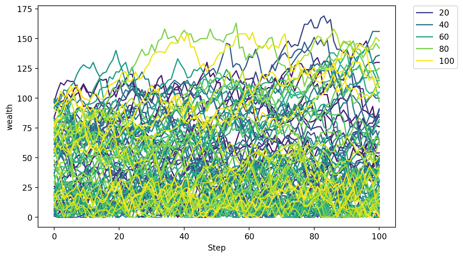
Now lets see what is each agents wealth over time

# First, we specify how large the image will be. In this case  in 8 inches by  5 inches. 
# We also specify that 200 dots per inch should be used. 

fig, ax = plt.subplots(figsize=(8,5), dpi=200)

# Use seaborn's lineplot to plot the data
# Set the data to agent_data DataFrame
# Set the x-axis to 'Step' column, y-axis to 'wealth' column, hue to 'AgentID' column
# Use 'viridis' color palette for the lines
# Set the axes to the created axes object
sns.lineplot(data=agent_data, x='Step', y='wealth', hue='AgentID', palette='viridis', ax=ax)

#Notice the hue argument. Hue is used to color the lines based on the values in the 'AgentID' column. 


# Add a legend to the plot
# Set the legend position to the upper left corner outside the plot
ax.legend(bbox_to_anchor=(1.05, 1), loc='upper left', borderaxespad=0)

<matplotlib.legend.Legend at 0x1190a0a50>

# Plot the wealth of the richest agent over time
fig, ax = plt.subplots(figsize=(8,5), dpi=200)
sns.lineplot(data=model_data, x='step', y='max_wealth')  # Use seaborn's lineplot to plot the data
plt.title('Wealth of the richest agent over time')  # Set the title of the plot

Text(0.5, 1.0, 'Wealth of the richest agent over time')

Task: describe what you see in the plots above

• Describe what you see in the two plots above

• First plot: what are the different lines in the first plot and why are they different from one another?

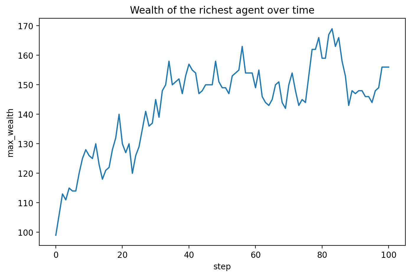
• Second plot: why is the trend in the second plot increasing?

Solution

Let’s describe what we see in the two plots:

1. First plot: Wealth of agents over time:

   • This plot shows multiple lines representing the wealth of individual agents over time. Each line corresponds to an agent (distinguished by colour using the AgentID column as the hue).

   • Why are the lines different?: The lines are different because agents accumulate or lose wealth at different rates depending on their interactions within the model. Some agents accumulate wealth quickly, while others may lose wealth or remain stagnant. The variety of lines indicates the diversity in wealth outcomes due to the randomness of agent interactions/ Each agent’s wealth fluctuates based on random interactions with other agents, which explains why some agents may end up with more wealth while others lose it.

2. Second plot: Wealth of the richest agent over time:

   • This plot tracks the maximum wealth in the system (held by the richest agent) at each step of the simulation.

   • Why is the trend increasing?: The trend is generally increasing because the richest agent continues to accumulate wealth over time. As agents interact and exchange wealth, the richest agent tends to become wealthier, which is a typical outcome in models of wealth distribution where resources concentrate among a few agents due to repeated advantageous interactions. The increasing trend reflects a common emergent property of such models, where wealth tends to become concentrated in the hands of fewer agents over time.

4.1.1.4: Random seeds

4.1.1.4.1: Run simulations without a random seed

When running simulations without a random seed, the results can vary significantly each time the model is executed. This is because the random number generator produces different sequences of random numbers, leading to different interactions and outcomes in the model.

Note that it can be called seed or random seed; it is the same thing.

# Let's make a small experiment to demonstrate the importance of setting a seed for reproducibility in simulations.
# Let's initialize the model two times without setting a seed (as we have done before)

# first model instance
model_1 = MoneyModel(100) 
# second model instance
model_2 = MoneyModel(100) 

# run the two models for 100 steps
for i in range(100):
    model_1.step()
    model_2.step()

# Save the results of the two models
model_data_1 = model_1.datacollector.get_model_vars_dataframe()
agent_data_1 = model_1.datacollector.get_agent_vars_dataframe()

model_data_2 = model_2.datacollector.get_model_vars_dataframe()
agent_data_2 = model_2.datacollector.get_agent_vars_dataframe()

# If you want to see the dataframe, we already learned how to display it before. Try it yourself.

# Let's plot the wealth of the richest agent over time for both models to compare them.

# Create a figure and axes object with specified size and dpi
fig, ax = plt.subplots(figsize=(8, 5), dpi=200)

# Plot the wealth of the richest agent over time for the first model
sns.lineplot(data=model_data_1, x='step', y='max_wealth', ax=ax, label='Model 1')
# Plot the wealth of the richest agent over time for the second model
sns.lineplot(data=model_data_2, x='step', y='max_wealth', ax=ax, label='Model 2')

# Set the title of the plot
plt.title('Wealth of the Richest Agent Over Time: Two Different Models')

# Set labels for the axes
ax.set_xlabel('Step')
ax.set_ylabel('Max Wealth')

# Add a legend to distinguish between the two runs
plt.legend()

# Show the plot
plt.show()

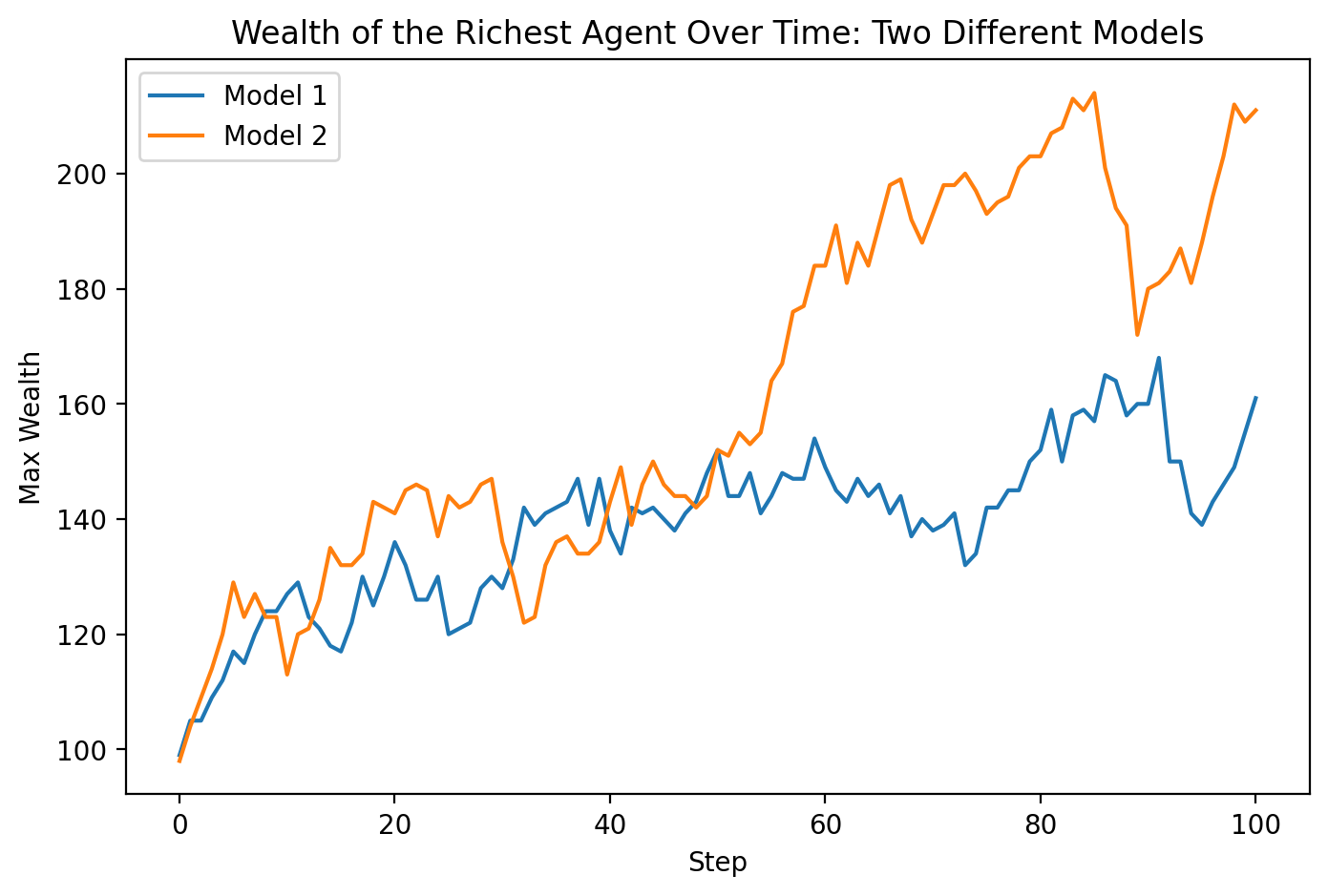
What is happening here? Why Are the Two Graphs Not the Same Although We Used the Same Model and the Same Parameters?

Although we used the same model and parameters, the two graphs differ because of the inherent randomness in agent interactions within the model. Each run produces different outcomes due to the stochastic nature of the model, where agents’ actions and interactions are determined by random choices.

4.1.1.4.2: Run simulations with a random seed

To ensure reproducibility in simulations, we can use a random seed. By setting a random seed, we can guarantee that the random processes in our model produce the same results every time we run the simulation. This is particularly useful for debugging and comparing different scenarios.

# Now we define the MoneyModel class again but this time with seed parameter for reproducibility. 
# Two changes are required: 
# The first is to add a seed parameter to the __init__ method of the MoneyModel class, 
# and the second is to pass the seed to the parent class's __init__ method (super().__init__(rng=seed))

class MoneyModel(Model):
    """A model with some number of agents."""
    def __init__(self, N, max_init_money=100, max_take_money=10, seed=None): # NOTE: added seed parameter for reproducibility.
                                                                                # seed = None disables the random seed, allowing for different runs to produce different results.
                                                                                # we will set the seed number later when we initialize the model
        # Initialize the model with a specified number of agents and parameters
        super().__init__(rng=seed) # NOTE: pass the seed to the parent class for reproducibility
        self.num_agents = N
        
        # Define the DataCollector to gather data during the simulation
        # Model-level metrics to be collected
        model_metrics = {
            "step": get_step_number,             # Collect the current step number of the model
            "agent_wealth": get_agents_wealth,   # Collect the wealth of all agents in the model
            "max_wealth": max_wealth,            # Collect the maximum wealth among all agents
            "richest_agent": richest,            # Collect the ID of the richest agent
        }
        # Agent-level metrics to be collected
        agent_metrics = {
            "wealth": "wealth"  # Collect the wealth attribute from each agent
        }
        # Note: Functions are referenced directly (e.g., get_step_number) while attributes are in quotes (e.g., "wealth")
        
        # Initialize the DataCollector with the defined model and agent metrics
        self.datacollector = DataCollector(model_reporters=model_metrics, agent_reporters=agent_metrics)

        # Create agents and add them to the model
        MoneyAgent.create_agents(self, self.num_agents, max_init_money, max_take_money)

        # Collect data at step 0 (initial state of the model)
        self.datacollector.collect(self)

    def step(self):
        """Advance the model by one step."""
        # Run the step for all agents in the model
        self.agents.shuffle_do("step") # Activate step for each agent in random order
        # Collect the model and agent data after running the step
        self.datacollector.collect(self)

# Let's now initialize the model 50 times with the SAME seed

# preparing the plot:
# Create a figure and axes object with specified size and dpi
fig, ax = plt.subplots(figsize=(8, 5), dpi=200)
# Set the title of the plot
plt.title('Wealth of the Richest Agent Over Time: 50 Different Runs')

# loop to run the model 50 times with the same seed
for rep in range(50):
    # Initialize the model with a specified number of agents and a fixed seed
    model = MoneyModel(100, seed=42)  # Try another seed value if you want ;)

    # Run each model for 100 steps
    for i in range(100):
        model.step()
    
    # Collect the model data
    model_data = model.datacollector.get_model_vars_dataframe()
    
    # Plot the wealth of the richest agent over time for this run
    ax = sns.lineplot(data=model_data, x='step', y='max_wealth')

# Show the plot
plt.show()

Observing the Effect of a Fixed Seed on Multiple Runs:

As you can see, all 50 curves are overlapped, which means the seed works. Every time we initiate a model with the same seed, we get the same curve. We did this 50 times and got the same result every time.

Task: random seed

• What if we want to fix the seed per repetition, so every repetition has a unique seed? Try to do this and see what you get.

# answer here

Solution

To fix the seed per repetition so that each run has a unique random seed, follow these steps:

1. Generate a unique seed for each repetition:

   • You can dynamically generate a seed for each run by using the repetition number (rep) as the seed. This ensures each run uses a different seed, leading to different outcomes for every repetition.

2. Modify the code:

   • Update the loop to provide a unique seed per repetition by setting seed=rep in the MoneyModel() initialization. This will give each run a different starting point for randomness.

3. Observe the results:

   • Since each run now uses a different seed, the resulting curves for the wealth of the richest agent will vary. Unlike when using the same seed, where all runs overlapped, these curves will now be distinct.

4. How does this work?:

   • Setting a fixed seed per repetition ensures you get different outcomes each time. However, it also means that every time you re-run the simulation with the same set of seeds, you will generate the same different curves each time. This is similar to not setting a seed at all, but the key difference is that you ensure consistency in the random outcomes. With no seed, different curves might be generated every time you run the simulation, whereas with a fixed seed, you ensure reproducibility of the different outcomes.

Notes:

1. Setting a unique seed per repetition is effectively similar to not setting a seed at all, in that you will get different outcomes each time. However, the advantage of setting a unique seed per repetition is that you ensure the same set of different outcomes each time you run the simulation. This guarantees that the different curves are reproducible.

2. In this case, using seed=rep ensures a consistent sequence of random events for each repetition, meaning the wealth curves will be distinct, but reproducible, every time the simulation is rerun.

4.1.1.5: Change the order in which agents step

4.1.1.5.1: Explore step orders

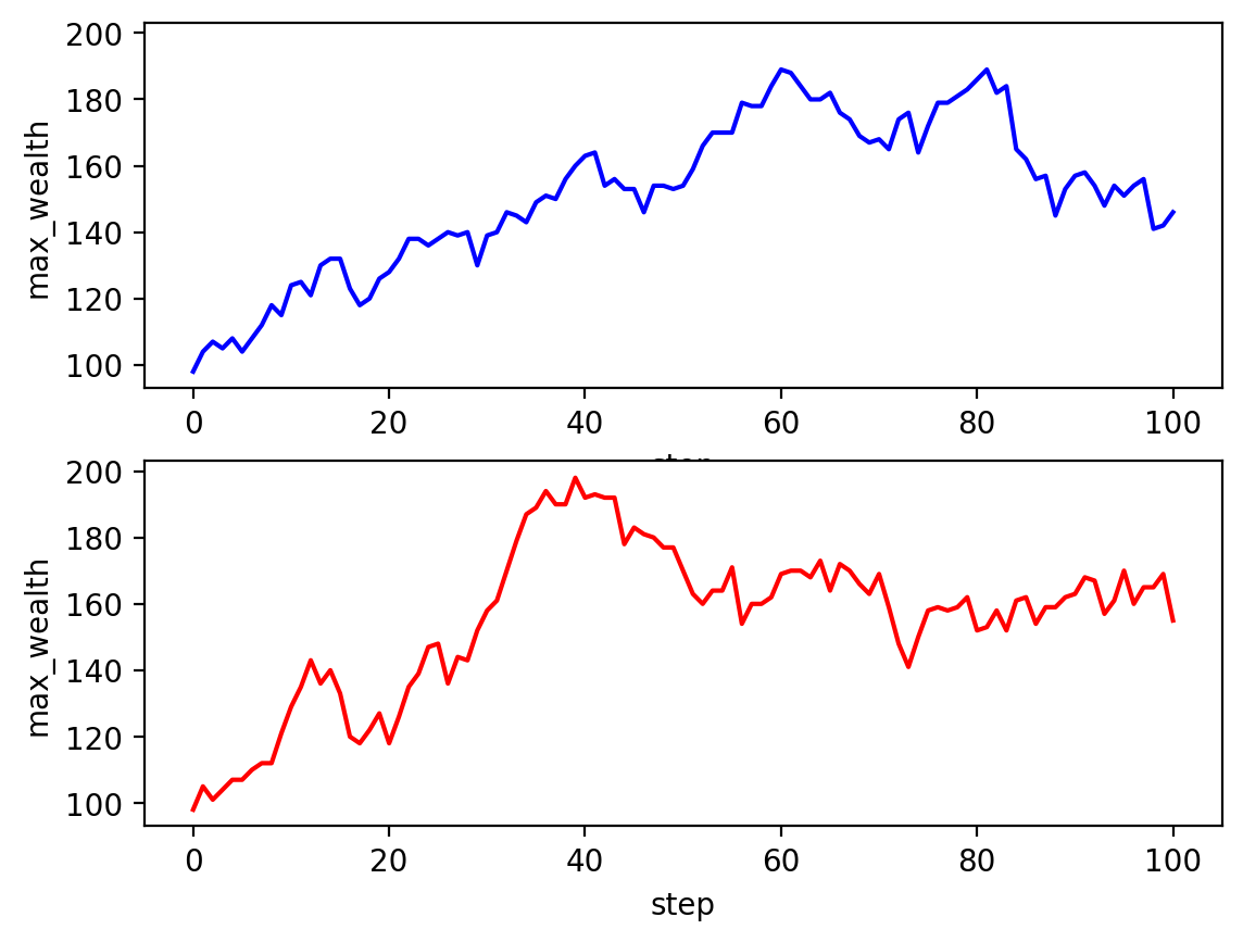
In this section, we explore the impact of different stepping orders on the model’s behaviour. Specifically, we compare a case which activates agents in a random order each step, with a case which activates agents in the order they were added to the model.

By running the model with each method and plotting the wealth of the richest agent over time, we can observe how the choice of order affects the simulation’s outcomes. This comparison helps us understand the significance of agent activation order in agent-based models.

Before turning to the tasks below, the activity that follows makes the stakes of this choice concrete. It runs the very same economy under a fixed activation order and under a reshuffled one, from the same random seed, so that any difference in the outcome can be attributed to the ordering alone.

Learning Activity: Who moves first?

see why the order in which agents are activated is a modelling decision, not a technical detail.

Two panels running the identical twelve-agent economy from the identical random seed, where a shared tray holds fewer bonus coins than there are agents, so the left panel keeps a fixed activation order while the right panel reshuffles it every tick.

Press Play, or advance one tick at a time with Step, and compare the wealth bars and the Gini coefficient beneath each panel.

agent wealthtook a coin this tickaverage wealth

self.agents.do("step")fixed order

Gini 0.00

self.agents.shuffle_do("step")random order

Gini 0.00

Play Step Reset tick 0 / 120

In Mesa 3.x this is exactly the difference between self.agents.do("step"), which activates the agents in the same fixed insertion order on every tick, and self.agents.shuffle_do("step"), which reshuffles that order each tick. When an agent's step reads and writes shared state, here, a limited resource claimed on a first-come basis, a fixed order bakes in a first-mover advantage for the earliest agents and manufactures inequality, while reshuffling each tick removes the artefact. Same seed, same draws: only the activation order differs.

The lesson to carry into the tasks is that agent activation order is a genuine modelling decision, not a technical afterthought: self.agents.do("step") fixes the order and can bake in a first-mover bias, whereas self.agents.shuffle_do("step") reshuffles it every tick and removes that artefact.

# Define a new model class with fixed order instead of random order
class MoneyModel_1(Model):
    """A model with some number of agents."""
    def __init__(self, N, max_init_money=100, max_take_money=10, seed=None):
        super().__init__(rng=seed)
        self.num_agents = N
        
        # Define the data collector, specifying which variables will be collected and how
        model_metrics = {
            "step": get_step_number,
            "agent_wealth": get_agents_wealth,
            "max_wealth": max_wealth,
            "richest_agent": richest,
        }
        agent_metrics = {
            "wealth": "wealth"
        }
        self.datacollector = DataCollector(model_reporters=model_metrics, agent_reporters=agent_metrics)
    
        # Create agents
        MoneyAgent.create_agents(
            model=self,
            n=self.num_agents,
            max_init_money=max_init_money,
            max_take_money=max_take_money
        )

        # Collect data at step 0 (initial state of the model)
        self.datacollector.collect(self)

    def step(self):
        """Advance the model by one step."""
        # Run the step
        self.agents.do("step") # Activate step for each agent in fixed order
        # Collect the model data after running the step
        self.datacollector.collect(self)

# Now let's run the model again with both random order and fixed order

# Initialize the models with the same number of agents and seed for reproducibility
model_1 = MoneyModel(100, seed=42)  # Using random order
model_2 = MoneyModel_1(100, seed=42)  # Using fixed order

# Run both models for 100 steps
for i in range(100):
    model_1.step()
    model_2.step()

# Save the data
# Get the Pandas DataFrame from the model using the table names defined in the model
model_data_1 = model_1.datacollector.get_model_vars_dataframe()  # Data from random order model
model_data_2 = model_2.datacollector.get_model_vars_dataframe()  # Data from fixed order model

# Get the agent-level data
agent_data_1 = model_1.datacollector.get_agent_vars_dataframe()  # Agent data from random order model
agent_data_2 = model_2.datacollector.get_agent_vars_dataframe()  # Agent data from fixed order model

# Uncomment the following if you would like to see the results in tabular form

# # Display the first few rows of the model data to inspect
# print("Model Data 1 (Random Order):")
# print(model_data_1.head())

# print("\nModel Data 2 (Fixed Order):")
# print(model_data_2.head())

# # Display the first few rows of the agent data to inspect
# print("\nAgent Data 1 (Random Order):")
# print(agent_data_1.head())

# print("\nAgent Data 2 (Fixed Order):")
# print(agent_data_2.head())

#create a plot of the richest agent over time, for  the two runs with different orders, on different plots
#Notice that we are using  subplots and we specify nroows to be 2. You can also use ncols for the number of columns. 
#You can also combine them for a matrix of graphs.
#Notice that we specify which axis is which, using (ax1,ax2)

fig, (ax1,ax2) = plt.subplots(nrows=2, sharey=True, dpi=200)

ax1 = sns.lineplot(data = model_data_1, x = 'step', y = 'max_wealth', color = 'blue', ax = ax1)
ax1 = sns.lineplot(data = model_data_2, x = 'step', y = 'max_wealth', color = 'red', ax = ax2)

Task 1: ordering

Explore the model with different values for starting money and money to take, and show the difference of the effect of the random seed and the order of agents activation

Part A: plot maximum wealth over time

Make a Plot of max wealth over time, with the model running using the same fixed seed:

• with fixed order and random order:

  • with low initial money, low money_to_take

  • with high initial money, low money_to_take

  • with low initial money, high money_to_take

  • with high initial money, high money_to_take

# answer here

Solution

Make a Plot of max wealth over time, with the model running using the same fixed seed:

In this task, you will compare the effects of different orders of activation on the max wealth of agents over time, using various initial conditions. Specifically, you will observe how the max wealth evolves with the following conditions:

1. Low initial money, low money to take.

2. High initial money, low money to take.

3. Low initial money, high money to take.

4. High initial money, high money to take.

Instructions:

1. Set up the model configurations:

   • You will define four configurations for the initial money and money to take. Use Python dictionaries to store these configurations for easy reference.

   • Example:

     configs = [
         {'init_money': 10, 'take_money': 5, 'label': 'Low Init, Low Take'},
         {'init_money': 1000, 'take_money': 5, 'label': 'High Init, Low Take'},
         {'init_money': 10, 'take_money': 100, 'label': 'Low Init, High Take'},
         {'init_money': 1000, 'take_money': 100, 'label': 'High Init, High Take'}
     ]
     

2. Iterate over the configurations and Run the model with both orders:

   • For each configuration in configs, run the model twice:

     • Once where agents are activated in random order. (Use self.agents.shuffle_do(‘step’))

     • Once where agents are activated in the order they were added. self.agents.do(‘step’)

     • You can iterate through the list of configurations using a for loop.

3. Collect data on max wealth over time:

   • For each configuration, run the model for 100 steps and collect the max wealth at each step. You can access the max wealth data using the datacollector.get_model_vars_dataframe() function, which stores the max wealth at each step.

   • Example code to run the model:

     model_data = model.datacollector.get_model_vars_dataframe()
     

4. Plot the results:

   • Use sns.lineplot() to plot the max wealth over time. You can overlay the results for both orders in the same subplot to compare them directly.

   • Set up subplots to visualise the results for each configuration. Each subplot should show the max wealth for both Random Order and Fixed Order on the same graph.

   • Example:

     sns.lineplot(data=model_data_ra, x='step', y='max_wealth', ax=ax, color='blue', label='Random Order')
     sns.lineplot(data=model_data_bs, x='step', y='max_wealth', ax=ax, color='red', label='Fixed Order')
     

5. Interpret the results:

   • Look at how max wealth evolves over time for each configuration.

     • Does the order of agent activation impact how wealth accumulates? Observe if the red and blue lines differ significantly in shape.

     • How do different initial money or money-to-take values affect wealth accumulation? Compare whether high initial money or high money-to-take accelerates wealth accumulation.

Hint:

• Use plt.subplots() to create subplots that compare each configuration.

Part B: plot a histogram of wealth

Make a histogram with seaborn that compares the distribution of wealth at the last tick, with the two orders

# answer here

Solution

Make a histogram with seaborn that compares the distribution of wealth at the last tick, with the two order

In this task, you will create a function to run the model and extract agent wealth data at the last tick (step 100). After collecting the wealth data for both random order and fixed order, you will use Seaborn to create a histogram that compares the wealth distribution for the two kinds of order.

Steps:

1. Create a function to run the model:

   • Write a function that accepts the order type (random or fixed), the number of agents, and other parameters such as initial money and the maximum amount agents can take. Inside the function:

     • Initialise the model using either MoneyModel for random or MoneyModel_1 for fixed.

     • Run the model for 100 steps using a loop. You can use a simple for loop:

       for i in range(100):
           model.step()
       

     • After running the model, collect the agent data using datacollector.get_agent_vars_dataframe() to access the wealth values of agents.

2. Set up the configuration:

   • Define a configuration with the initial money and maximum money to take for the agents. For example:

     config = {'init_money': 100, 'take_money': 50}
     

   • This configuration will be used to run the model with both orders.

3. Run the model for both orders:

   • Call the function twice, once for random and once for fixed, to collect the wealth data at step 100 for both orders. Use .loc[100, 'wealth'] to extract the wealth values at the last tick:

     wealth_ra_t100 = agent_data_ra.loc[100, 'wealth']
     wealth_bs_t100 = agent_data_bs.loc[100, 'wealth']
     

4. Plot the wealth distribution:

   • Use Seaborn’s sns.histplot() to create a histogram comparing the wealth distribution at step 100 for both orders:

     • Plot for Random Order: Use blue colour and add a KDE curve to smooth the distribution.

     • Plot for Fixed Order: Use red colour and another KDE curve.

   • Example:

     sns.histplot(wealth_ra_t100, color='blue', label='Random Order', kde=True)
     sns.histplot(wealth_bs_t100, color='red', label='Fixed Order', kde=True)
     

5. Add labels and a legend:

   • Use plt.title() to set the plot title and plt.xlabel() and plt.ylabel() to label the axes:

     plt.title('Wealth Distribution at Step 100 for Both Orders')
     plt.xlabel('Wealth')
     plt.ylabel('Number of Agents')
     

   • Add a legend using plt.legend() to distinguish the two kinds of order.

6. Display the plot:

   • Finally, call plt.show() to display the plot and visualise the wealth distribution comparison.

You have now seen inequality appear from fair exchanges, watched a single seed replay the same history, and seen how the activation order can tip the outcome. Before moving on to the open exercises, it is worth pausing to ask what this simple economy is really telling us, and what it quietly leaves out.

Reflection questions

1. Every exchange in this model is symmetric: giver and receiver are chosen by the same fair random rule, and no money is created or destroyed. So why does inequality appear at all, instead of everyone staying near the average?

2. Running the model with the same random seed reproduces exactly the same final distribution every time. Does that make the outcome inevitable, or is it still random? What is the difference between “determined by the seed” and “predictable in advance”?

3. Name two forces from real economies that this model leaves out (for example production, saving, inheritance, wages, or taxation). For each, predict whether adding it would raise or lower the Gini coefficient, and briefly say why.

Solution

1. Inequality here is emergent, not built in. Money performs a random walk between agents, and a random walk has no restoring force pulling wealth back towards the mean. An agent that drifts down to zero simply stops giving, while agents above the mean keep redistributing, so the distribution spreads into a skewed, roughly exponential shape. Fairness in a single exchange does not guarantee equality in the aggregate.

2. Both are true at once. The trajectory is fully determined by the seed, so it is reproducible, but it is not predictable without actually running the model: there is no shortcut formula that gives one agent’s final wealth. This is the usual situation in agent-based modelling, where a macro pattern is a deterministic consequence of the micro rules yet can only be found by simulating them.

3. Adding saving (agents keep a fraction rather than always giving) tends to lower the Gini, because it damps the random walk. Adding inheritance or compounding returns, where wealth begets wealth, tends to raise the Gini sharply, because it introduces the positive feedback this model lacks. Taxation with redistribution lowers it. The wider point is that the baseline model already produces substantial inequality from nothing but chance, so any real mechanism should be judged by how much it adds to, or subtracts from, that baseline.

The lesson to carry into the exercises is that a model can generate a strong, non-obvious pattern from a completely fair and simple rule, and that reading such a pattern always means asking what the model includes and what it omits.

Exercises

Exercise 1: create a complex but useful plot

Make a plot in which you show the average agent wealth and the standard deviation of agent wealth over time? You may use the base model.

Hint: the agent_data is a MultiIndex data frame and seaborn has boxplot feature

• method: sns.boxplot

• data: agent_data

• y axis: wealth

• x axis: step

# answer here

Solution

In this exercise, you will create a boxplot that shows the distribution of agent wealth over time. A boxplot is a useful way to visualise how wealth is distributed at each simulation step.

Steps:

1. Run the model for 100 steps:

   • Use the base model to run the simulation for 100 steps. You can use random shuffling for steps. The data you collect will include the wealth of each agent at every step.

2. Create a boxplot:

   • After running the model, use Seaborn’s sns.boxplot() function to create the plot. On the x-axis, plot the step number, and on the y-axis, plot the wealth of agents:

     sns.boxplot(data=agent_data.reset_index(), y='wealth', x='Step')
     

Exercise 2: add an attribute to the agent

1. Choose an attribute: Think of an attribute that could be relevant to the agents. An example could be:

   • job: to represent the type of job the agent has.

2. Implement the attribute: Add the chosen attribute to the MoneyAgent class. Initialise it in the constructor (__init__ method) and update the step method if necessary.

3. Add it to the data collector and run the model.

4. Display the agent data table to see the attributes

# answer here

Solution

In this exercise, you will extend the agent by adding a new attribute. For this task, we will add the attribute job to represent the type of job each agent has. You will then display the agent data table to observe the attributes of each agent over time.

Steps:

1. Choose an attribute:

   • For this exercise, we will add the job attribute to the agent. The possible job types will be 'farmer', 'merchant', or 'banker', which will be randomly assigned to each agent.

2. Implement the attribute:

   • In the MoneyAgent class, add the job attribute in the __init__ method:

     # New: Add 'job' attribute, randomly assigned from a list of jobs
     self.job = self.random.choice(['farmer', 'merchant', 'banker'])
     

3. Add the attribute to the DataCollector:

   • In the MoneyModel class, update the DataCollector to collect the job attribute, along with wealth:

     # New: Add 'job' attribute to the DataCollector
     agent_reporters={"wealth": "wealth", "job": "job"}
     

4. Run the model:

   • Run the model for 100 steps and collect the data. The new attribute job will be recorded for each agent at every step.

5. Display the agent data table:

   • After running the model, you will display the agent data table to see the collected attributes.

Exercise 3: add and visualise a function

1. Choose a function: Think of a function that can provide useful data about the agents or the model. An example could be:

   • Total wealth of all agents.

2. Implement the function: Define the function outside the model class and include it in the DataCollector.

3. Visualise the data: Use a visualisation method (e.g., line plot, histogram) to visualise the collected data.

# answer here

Solution

In this exercise, you will add a function to calculate and visualise useful data about the agents or the model. For this task, we will calculate the total wealth of all agents at each step and visualise how it changes over time.

Steps:

1. Choose a function:

   • We will create a function called compute_total_wealth to calculate the total wealth of all agents at each step. This function will sum the wealth of every agent in the model.

2. Implement the function:

   • Define the compute_total_wealth function outside the model class:

     def compute_total_wealth(model):
         """Returns the total wealth of all agents in the model."""
         return sum([agent.wealth for agent in model.agents])
     

   • Add the function to the DataCollector in the MoneyModel class:

     # New: Add 'total_wealth' function to the DataCollector
     self.datacollector = DataCollector(
         model_reporters={"step": get_step_number, "total_wealth": compute_total_wealth}
     )
     

3. Run the model and display the model dataframe:

   • Run the model for 100 steps and display the model data frame

4. Visualise the data:

   • Use Seaborn’s sns.lineplot() to create a line plot that shows how the total wealth of all agents changes over time:

     sns.lineplot(data=model_data, x='step', y='total_wealth')
     

Exercise 4: implement a different activation order

1. Search for an ordering technique: Look into the Mesa documentation to find different types of ordering techniques. Some examples include:

   • In stages: Runs all agents in a particular order.

   • At same time: Steps all agents simultaneously.

   • Fixed order: Steps all agents in the same fixed order.

2. Implement the orders: Replace the random order in your model with the new orders.

3. Run the model with all three orders and compare results of the maximum wealth at each time steps. Observe any differences in the simulation outcomes and comment on how the choice of ordering technique affects the results.

# answer here

Solution

In this exercise, you will implement and compare three different orders: Random, Simultaneous, and Staged. You will run the model using each order, collect the max wealth of agents, and compare the results.

Steps:

1. Search for the different orders:

   • We will use three different orders from the Mesa library:

     • Random: Steps agents in random order.

     • Simultaneous: Steps all agents simultaneously.

     • Staged: Steps agents in a specified sequence (in this case, all agents perform their actions in the same order).

2. Implement the orders:

   • The MoneyModel class is updated to accept a order_type parameter. Depending on this parameter, the appropriate order is assigned in the model at the self.step() function:

     if self.order_type == "Random":
         self.agents.shuffle_do("step")
     elif self.order_type == "Simultaneous":
         self.agents.do("step")
         self.agents.do("advance")
     elif self.order_type == "Staged":
         for stage in ["step"]:
              self.agents.do(stage)
     

3. Run the model:

   • We will create a run_model function that takes in the order type as a parameter and runs the model for 100 steps. For each order, the max wealth of all agents is tracked and returned as a DataFrame:

     def run_model(order_type):
         model = MoneyModel(N=100, max_init_money=100, max_take_money=10, order_type=order_type)
         for i in range(100):
             model.step()
         return model.datacollector.get_model_vars_dataframe()
     

4. Run the models for each order:

   • The model will be run for each of the three orders, and the collected data will be stored:

     random_data = run_model("Random")
     simultaneous_data = run_model("Simultaneous")
     staged_data = run_model("Staged")
     

5. Prepare the data for comparison:

   • To compare the results, a new column will be added to each dataset to indicate the order type. The data is then concatenated into a single DataFrame:

     random_data['Order'] = 'Random'
     simultaneous_data['Order'] = 'Simultaneous'
     staged_data['Order'] = 'Staged'
     
     comparison_data = pd.concat([random_data, simultaneous_data, staged_data])
     

6. Visualise the results:

   • Use Seaborn’s lineplot() to compare the max wealth of agents over time for each order. This will help you understand how the choice of order affects the dynamics of wealth distribution:

     sns.lineplot(data=comparison_data, x='step', y='max_wealth', hue='Order')
     

Exercise 5: change the behaviour of the agents

1. Modify the behaviour of the agents so that agents can give money even if they don’t have enough, resulting in debt.

2. visualise:

   • the total wealth results

   • the maximum wealth at each time step

# answer here

Solution

In this exercise, you will modify the behaviour of agents so that they can give money even if they don’t have enough, resulting in debt. After modifying the behaviour, you will visualise the total wealth of all agents and the maximum wealth at each time step.

Steps:

1. Modify the behaviour of agents:

   • In the MoneyAgent class, update the step method so that agents can give money even if they don’t have enough, which results in negative wealth (debt):

     other_agent.wealth -= money_to_take
     self.wealth += money_to_take
     

2. Update the MoneyModel class:

   • Add max_wealth and total_wealth reporters to the DataCollector in the MoneyModel class so that both total wealth and maximum wealth are tracked:

     self.datacollector = DataCollector(
         model_reporters={"total_wealth": compute_total_wealth, "max_wealth": max_wealth}
     )
     

3. Run the model:

   • Run the model for 100 steps with the updated agent behaviour. Use the run_model_with_debt function to simulate the model:

     model_data_with_debt = run_model_with_debt("Random")
     

4. Visualise the results:

   • Use a line plot to visualise the total wealth of all agents over time. This will help you observe how the overall wealth in the system changes when agents can go into debt:

     sns.lineplot(data=model_data_with_debt, x='step', y='total_wealth')
     

   • Additionally, use a line plot to visualise the maximum wealth of agents at each time step. This will show the fluctuations in wealth of the richest agents over time:

     sns.lineplot(data=model_data_with_debt, x='step', y='max_wealth')
     

Exercise 6: add a grid, extend agent behaviour, and visualise the dynamics

It’s time now to introduce a spatial dimension. In this exercise, you will modify the basic model to include a grid, allowing agents to move around and interact with others.

Task:

1. Add a Grid to the Model:

   • Modify your model to include a grid where agents can be placed. Use Mesa’s MultiGrid or SingleGrid to represent the environment.

   • Ensure that agents are placed on the grid at random positions when the model is initialised.

2. Implement Agent Movement:

   • Define a move method for the agents. This method should allow an agent to move to a neighboring cell on the grid.

   • Use the Moore neighborhood (which includes diagonal moves) to determine possible moves. Ensure that the agent doesn’t move to its current position.

3. Modify Agent Behaviour for Interaction:

   • Adjust the agent’s step method so that after moving, the agent interacts with others in the same cell.

   • Implement a mechanism where an agent gives wealth to another agent in the same cell, but only if the agent has wealth greater than zero.

4. Visualise the model’s dynamics:

   • Create a visualisation of your model to observe how agents move and interact on the grid over time.

   • You may use the visualisation code we introduced in the Mesa tutorial as a starting point

Hints:

• Consider how to randomly select a new position within the neighborhood for the agent to move to.

• Think about how to check for other agents in the same cell after moving and how to handle the wealth exchange.

• We have performed a similar task during the Mesa tutorial. Try first to complete the exercise without looking at the Mesa tutorial. However, if you get stuck, you may refer to the solution as needed.

# answer here

Solution

In this exercise, you will add a spatial dimension to the model by introducing a grid where agents can move and interact with others. You will also visualise the model’s dynamics using an animation to observe how agents’ wealth changes over time.

Steps:

1. Add a Grid to the Model:

   • Use Mesa’s MultiGrid to create a grid for agents to move around. When the model is initialised, agents will be randomly placed on the grid:

     self.grid = MultiGrid(width, height, True)  # Grid with wrap-around (toroidal)
     

2. Implement Agent Movement:

   • Define a move method for the agents to allow them to move to a neighboring cell using the Moore neighborhood (including diagonal moves):

     possible_moves = self.model.grid.get_neighborhood(self.pos, moore=True, include_center=False)
     new_position = self.random.choice(possible_moves)
     self.model.grid.move_agent(self, new_position)
     

3. Modify Agent Behaviour for Interaction:

   • After moving, agents will interact with others in the same cell. If the agent has wealth greater than zero, they will give 1 unit of wealth to another agent in the same cell:

     if self.wealth > 0:
         self.wealth -= 1
         other_agent.wealth += 1
     

4. Visualise the Model’s Dynamics:

   • Use matplotlib and FuncAnimation to create an animated visualisation of the agents moving and interacting on the grid. You can observe how agents with wealth (represented by red circles) move and interact with other agents (grey circles representing agents with zero wealth):

     anim = FuncAnimation(fig, update, frames=100, repeat=False, interval=200)
     HTML(anim.to_jshtml())
     

   • See the Mesa tutorial for an example

Exercise 7: write the simple economy model yourself

Looking at an existing model without practicing the actual code writing often leads to false feeling of understanding. Therefore, this exercise is designed to help you confirm your understanding of what constitutes an ABM model.

Task: write the code for the simple economy model from scratch, without looking at the provided code above. You may use the Mesa documentation as a resource during the coding process. However, if you find yourself stuck and unable to proceed, you may refer to the provided model to help you move forward. You may also use the flowchart you created earlier

Please do not skip this exercise.

# answer here

Completion and reflection

Before you finish, confirm that you can:

• Run the base model with a fixed seed and explain one source of inequality.

• Use model- and agent-level tables to support a claim with a plot or summary statistic.

• Change activation order or one behavioural rule and compare it with the baseline.

• Record the seed, parameter values, and interpretation needed to reproduce your result.