

1.2.5: Simulation experiments#
Once the model has been verified and validated, the modeller uses it to answer the research question. Nikolic, van Dam and Lukszo describe this as the experimentation stage: the model is run under controlled conditions to generate the data that will be analysed [1]. A single run rarely answers a research question on its own. What answers it is a designed set of runs in which the inputs are varied systematically and the outputs are compared across the variations [1].
1.2.5.1: Designing a simulation experiment#
A good experiment is set up before the runs begin, not chosen afterwards to fit a story. Designing the comparison in advance determines what evidence the runs can provide. The modeller should name the response metrics, decide whether early warm-up steps are discarded, specify a stopping rule, and state which inputs remain fixed while others vary. These decisions prevent a parameter sweep from becoming an undirected search for an attractive graph. They also make the resulting dataset interpretable: differences between scenarios can be traced to planned changes rather than undocumented alterations in the run conditions.
The ingredients of a well-designed experiment are:
What the modeller expects to find, and why, stated before the runs so the experiment can confirm or contradict it [1].
A reference configuration that every other run is compared against, so the effect of each change can be isolated [1].
Which parameters will be changed, and the range of values each will take [1].
How many times each configuration is run with different random seeds, so results are averages rather than single observations [1].
How long each run lasts, chosen so the behaviour of interest has time to appear and settle [1].
The distinct configurations to be compared, each described clearly enough to be reproduced [1].
1.2.5.2: Parameter sweeps and sensitivity analysis#
The variables, ranges, and scenarios listed above do not run themselves; the parameter sweep is the mechanism that realises them. The standard way of exploring the input space is the parameter sweep: the model is run across a range of values for one or more parameters, and the output is recorded for every combination. A full factorial sweep covers every combination in a defined grid; when that is impractical, the modeller samples a smaller set of combinations [1]. The same machinery supports sensitivity analysis, which asks how strongly each parameter affects the outputs and is the standard way to tell which assumptions the conclusions depend on [2].
The activity below lets you run such a sweep by hand: a single shot at a fixed release angle is mostly luck, but replicating at that angle and then sweeping the angle across its range reveals how the success rate depends on the setting, and which settings are robust to noise rather than fragile.
Reading that curve is a sensitivity analysis in miniature: it shows not just which release angle is best but how steeply the outcome depends on it, so a robust setting near the peak can be told apart from the fragile settings on the flanks.
1.2.5.3: Why replication is non-negotiable#
Because these models usually include randomness, the same setting will not give the same output twice. Replication is therefore a golden rule: run each configuration several times and summarise with statistics such as means and standard deviations [1]. A claim from one run is a claim about a single history of the model, not about what it generally produces: one run is one possible history, and it could land almost anywhere, so only by repeating the run many times does a stable estimate emerge from the noise. Results are therefore reported with their spread (error bars or confidence intervals), and all the experiments are reported, not only the ones that came out well [1]. The modeller also has to be explicit about which metrics are collected and why each matters [1].
The activity below makes this concrete. Each blue dot is one run of a model whose output varies, and as the replications add up the estimate settles and the confidence interval shrinks: the visual form of why we report a spread rather than a single number.
One run could have told almost any story; the average only became trustworthy once it was backed by many runs and reported with its spread. This is why a result from a stochastic model is a distribution to be summarised, never a single number to be quoted.
With the method in place, it helps to see it operate on a concrete case. The traffic model puts every ingredient to work at once.
1.2.5.4: The traffic example#
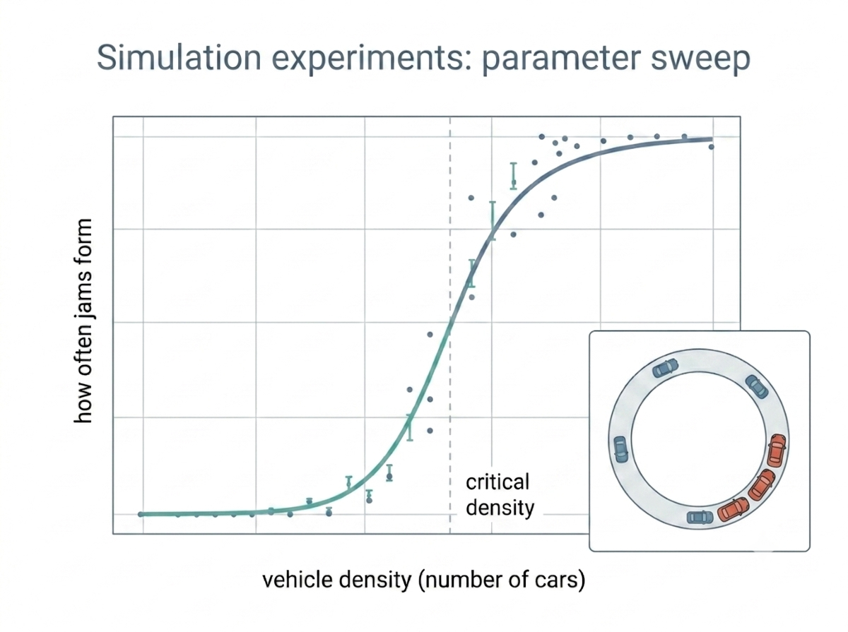
Fig. 9 Figure 1.9 A parameter sweep over vehicle density. Each point is averaged across several replications with different random seeds; jams are rare below a critical density and become frequent above it, revealing a threshold in how often congestion forms.#
For the traffic model, the question is how jams form on a road with no external cause. The most natural parameter to vary is the number of vehicles on the loop, because real traffic becomes unstable above a certain density [3]. The baseline is a low density at which traffic flows freely, and the experiment sweeps the vehicle count upward from there. With several replications at each count, the sweep produces a dataset showing how often jams form, how long they last, and how the fraction of vehicles at full speed depends on density.
Other parameters can be varied at the same time. Acceleration and deceleration affect how quickly drivers respond to the gap ahead, and sweeping across these is exactly the sensitivity analysis introduced above, applied here to show how strongly jam formation depends on driving behaviour [3][2]. The hardest part is then the data analysis: finding patterns in the output and connecting them back to the vehicles’ rules and interactions [1]. The analysis asks what the patterns mean: if jams begin to form at a particular density and grow rapidly above it, the model is showing the threshold seen in empirical traffic data, and if that threshold shifts when deceleration changes, the model is showing how driver behaviour and density interact [3]. Connecting these observations back to the vehicles’ rules is what turns the output into an answer to the research question [1].
That interpretive step is a skill in its own right, and the activity below gives you practice with it: each row reports one thing a sweep showed, and you decide what it tells you about the model.
Naming each pattern a sweep reveals, then tracing it back to the vehicles’ rules, is the analytical step that separates merely running experiments from interpreting them.
1.2.5.5: Judging when a claim has enough evidence#
The traffic case showed the method producing a specific answer; the same discipline lets you judge any stochastic result, your own or someone else’s. Knowing that one run is not a result is only half the skill; the other half is judging when a claim rests on enough evidence to be believed. A trustworthy claim from a stochastic model comes from several replications, is reported with its spread, and includes every run rather than only the tidy ones that fit the story. This judgement protects you both when you report your own results and when you read someone else’s. In the activity below, judge each case for whether the evidence is strong enough, weighing each one against those three requirements.
The trustworthy cases all shared the same discipline: several replications, the spread reported, and every run included. Selecting the run that fits the story is exactly what a careful simulation experiment refuses to do.
With a designed set of experiments run and analysed, the final stage of the cycle carries these results back to the real system that raised the question, covered next in 1.2.6: Using the model.
Key takeaways#
Key takeaways
A research question is answered by a designed set of runs, not a single run: fix the hypothesis, baseline, variables, replications, duration, and scenarios in advance.
Because the model is random, run several replications per setting and report results with their spread, not single numbers.
A parameter sweep maps how outputs depend on inputs and doubles as sensitivity analysis; the hard part is interpreting the patterns and tracing them back to the rules.